
【Class】Stanford CS149 Parallel Computing
学习一下“金字塔尖”课程,全英文不知道能不能看懂😭(自己的课程倒头就睡,别人的课程逐帧学习😜) The goal of this course is to provide a deep understanding of the fundamental principles and engineering trade-offs involved in designing modern parallel computing systems as well as to teach parallel programming techniques necessary to effectively utilize these machines. Because writing good parallel programs requires an understanding of key machine performance characteristics, this course will cover both parallel hardware and software design
课程
2023年课程视频 + 2025年PPT
课程视频
Stanford CS149 I Parallel Computing I 2023 I Kayvon Fatahalian and Kunle Olukotun - YouTube
课程信息
gfxcourses.stanford.edu/cs149/fall25/
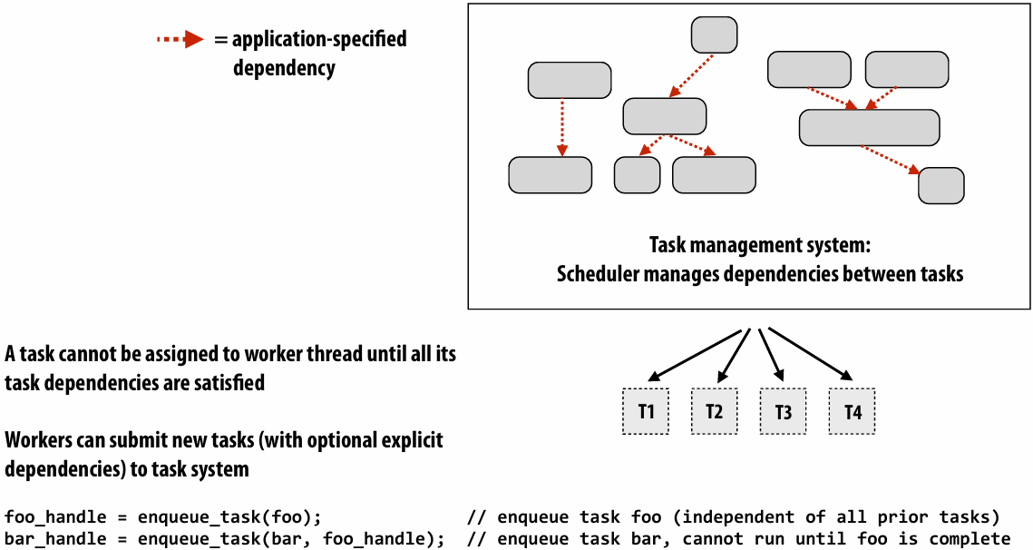
Programming Assignments
Written Assignments

Lecture 1: Why Parallelism? Why Efficiency?
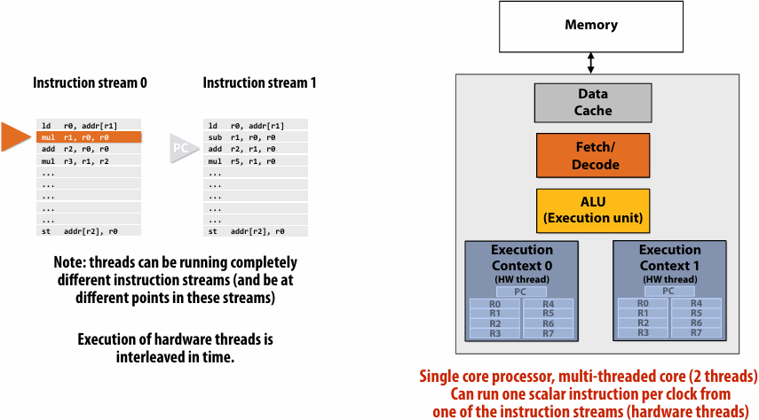
A parallel computer is a collection of processing elements that cooperate to solve problems quickly
collection of processing elements: We’re going to use multiple processing elements to get it
quickly: We care about performance, and we care about efficiency
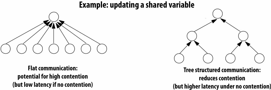
Speedup
One major motivation of using parallel processing: achieve a speedup
For a given problem:
Communication limited the maximum speedup achieved
Minimizing the cost of communication improved speedup
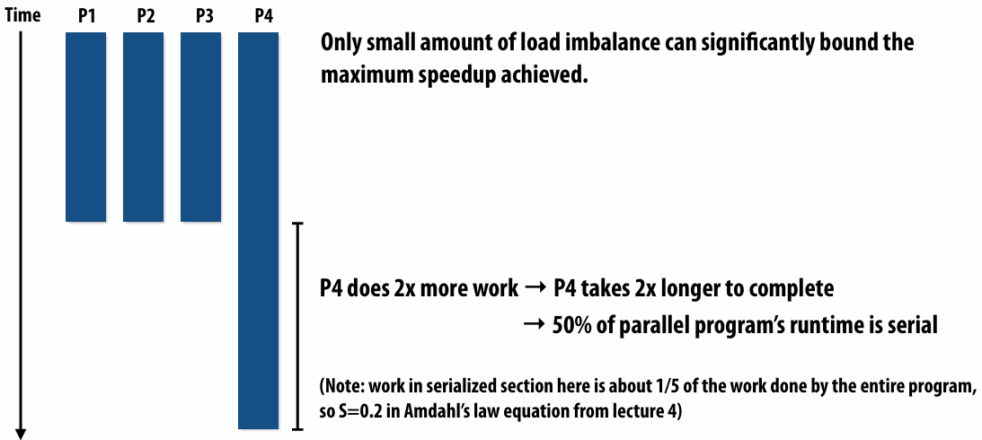
Imbalance in work assignment limited speedup
Improving the distribution of work improved speedup
Communication costs can dominate a parallel computation, severely limiting speedup
Course theme
Course theme 1
Designing and writing parallel programs … that scale!
Parallel thinking
1.Decomposing(分解) work into pieces that can safely be performed in parallel
2.Assigning work to processors
3.Managing communication / synchronization(同步) between the processors so that it does not limit speedup
Abstractions(抽象) / mechanisms(机制) for performing the above tasks
Writing code in popular parallel programming languages
Course theme 2
Parallel computer hardware implementation: how parallel computers work
Mechanisms used to implement abstractions efficiently
1.Performance(性能) characteristics of implementations
2.Design trade-offs(权衡): performance vs. convenience vs. cost
Why do I need to know about hardware?
1.Because the characteristics of the machine really matter
2.Because you care about efficiency and performance
Course theme 3
Thinking about efficiency
FAST != EFFICIENT
Just because your program runs faster on a parallel computer, it does not mean it is using the hardware efficiently
Programmer’s perspective: make use of provided machine capabilities
HW(HardWare) designer’s perspective: choosing the right capabilities(功能) to put in system (performance / cost, cost = silicon area?, power?, etc.)
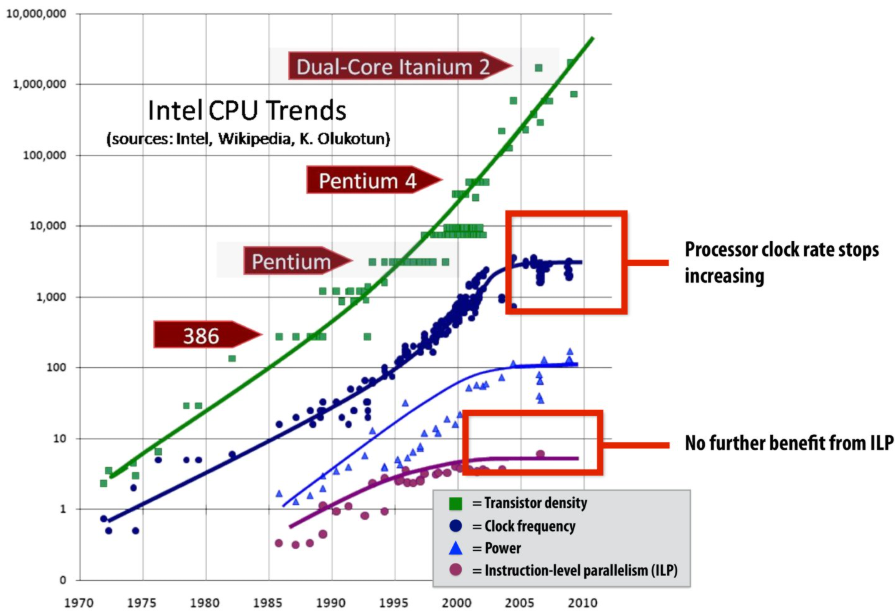
Until ~ 20 years ago: two significant reasons for processor performance improvement
1.Exploiting(利用) instruction-level(指令级) parallelism(superscalar(超标量) execution)
2.Increasing CPU clock frequency
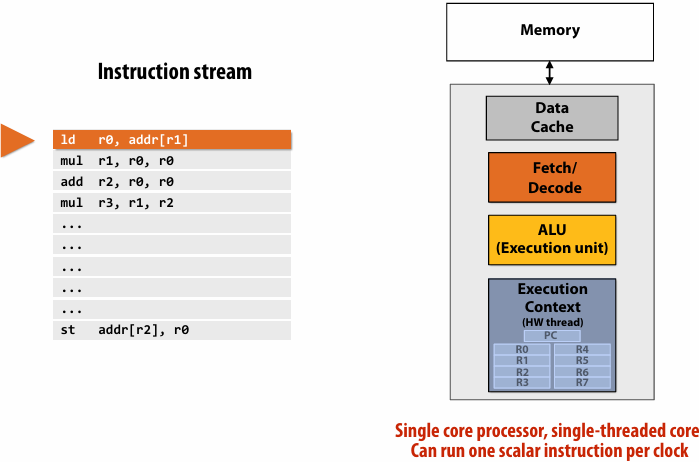
What is a program?(from a processor’s perspective)
A program is just a list of processor instructions
What is an instruction?
It describes an operation for a processor to perform
Executing an instruction typically modifies the computer’s state
computer’s state: the values of program data, which are stored in a processor’s registers or in memory
What does a processor do?
A processor executes instructions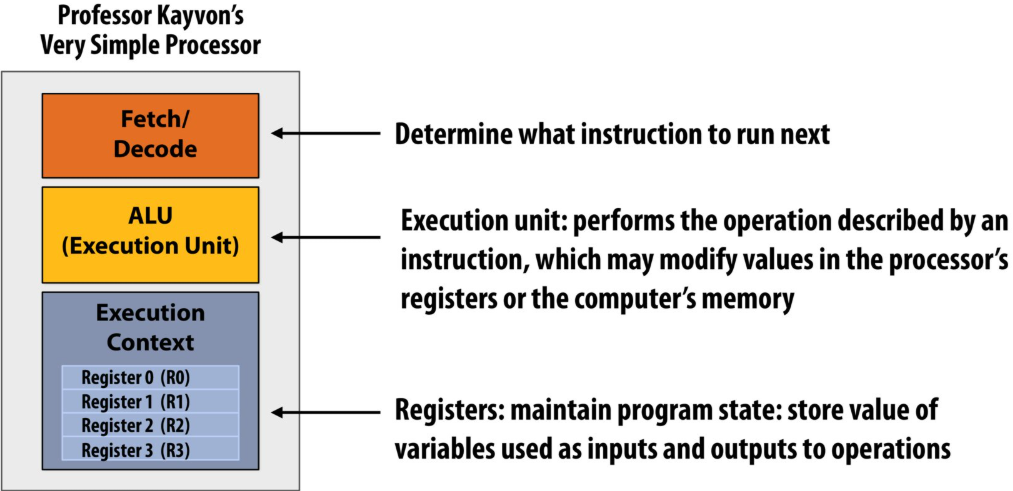
executes one instruction per clock
Superscalar execution: processor automatically finds (Or the compiler finds independent instructions at compile time and explicitly encodes dependencies in the compiled binary(二进制文件)) independent instructions in an instruction sequence and executes them in parallel on multiple execution units
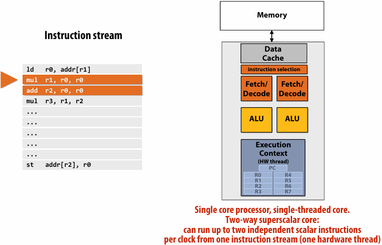
Superscalar processor
This processor can decode and execute up to two instructions per clock
Diminishing(递减) returns(收益) of superscalar execution
Most available ILP(instruction-level parallelism) is exploited by a processor capable of issuing(发出) four instructions per clock(Little performance benefit from building a processor that can issue more)
ILP tapped out(已达极限) + end of frequency scaling(扩展)
The “power wall”
Power consumed by a transistor:

Static power: transistors burn power even when inactive due to leakage
High power = high heat
Power is a critical design constrant in modern processors
Maximum allowed frequency determined by processor’s core voltage
Single-core performance scaling
The rate of single-instruction stream performance scaling has decreased(almost to zero)
1.Frequency scaling limited by power
2.ILP scaling tapped out
Architects are now building faster processors by adding more execution units that run in parallel(Or units that are specialized for a specific task: like graphics, or audio / video playback)
Software must be written to be parallel to see performance gains. No more free lunch for software developers!
| 特性 | 指令级并行(ILP) | 手动编写的并行(TLP/DLP) |
|---|---|---|
| 负责人 | 硬件(CPU) | 程序员(软件) |
| 代码形式 | 普通的顺序代码 | 特殊的多线程/向量化代码 |
| 程序员负担 | 零负担 (自动提升) | 负担沉重 (需设计架构、调试并发 BUG) |
| 并行规模 | 很小 (通常每个时钟周期几条指令) | 很大 (可以扩展到成千上万个核心) |
| 限制因素 | 指令间的依赖关系、电路复杂度 | 算法的可拆分性、同步开销 (阿姆达尔定律) |
| 粒度 | 极细(指令级)。处理的是加法、乘法、访存等最基本的指令 | 较粗(线程级或任务级)。程序员将一个大任务拆分成多个子任务(例如:处理图像时,把图像分成四块,交给四个核心处理) |
| 实现方式 | 通过流水线(Pipelining)、乱序执行(Out-of-Order Execution)、多发射(Multiple Issue)和分支预测等技术 | 程序员需要考虑如何拆分任务、如何处理线程间的同步(锁、信号量)、如何避免死锁以及如何进行数据交换 |
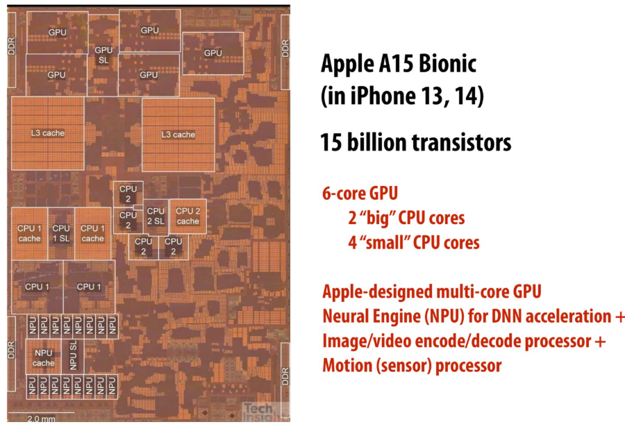
Mobile parallel processing
Power constraints also heavily influence the design of mobile systems
What is a big concern in all computing?
Power
Two reasons to save power
Run at higher performance for a fixed(固定的) amount of time
Power = heat If a chip gets too hot, it must be clocked down(减低频率) to cool off(Another reason: hotter systems cost more to cool)
Run at sufficient performance for a longer amount of time
Power = battery Long battery life(续航时间) is a desirable feature in mobile devices
Specialized processing is ubiquitous in mobile systems
 Motion(sensor)(运动(传感器))
Parallel + specialized HW
Modern systems not noly use many processing units, but also utilize specialized processing units to achieve high levels of power efficiency
Achieving efficient processing almost always comes down to(归结为) accessing data efficiently
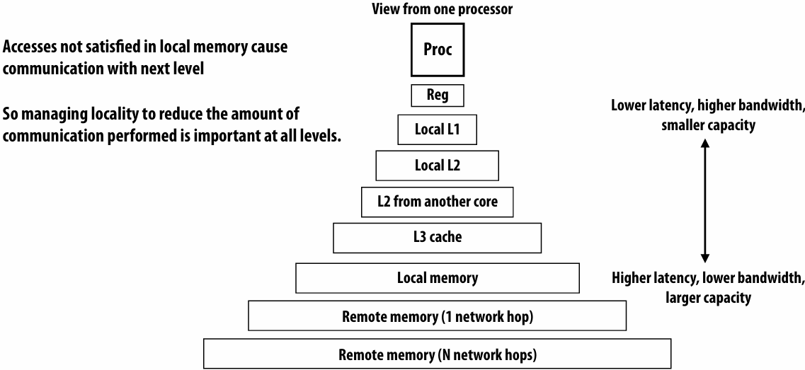
What is memory?
A program’s memory address space
A computer’s memory is organized as an array of bytes
Each byte is identified by its “address” in memory(its position in this array)(We’ll assume memory is byte-addressable)
Load: an instruction for accessing the contents of memory
Memory access latency(延迟)
The amount of time it takes the memory system to provide data to the processor
Stalls(停顿)
A processor “stalls” (can’t make progress) when it cannot run the next instruction in an instruction stream because future instructions depend on a previous instruction that is not yet complete
Accessing memory is a major source of stalls
Memory access times ~ 100’s of cycles, is a measure of latency
What are caches?
- A cache is a hardware implementation detail that does not impact the output of a program, only its performance
- Cache is on-chip storage that maintains a copy of a subset(子集) of the values in memory
- If an address is stored “in the cache” the processor can load/store to this address more quickly than if the data resides(驻留) only in DRAM
- Caches operate at the granularity(粒度) of “cache lines”
There are two forms of “data locality(局部性)” in this sequence:
Spatial(空间) locality: loading data in a cache line “preloads(预加载)” the data needed for subsequent(后续) accesses to different address in the same line, leading to cache hits
Temporal(时间) locality: repeated accesses to the same address result in hits
Caches reduce length of stalls(reduce memory access latency)
Processors run efficiency when they access data that is resident(驻留) in caches
Caches reduce memory access latency when processors accesses data that they have recently accessed!(Caches also provide high bandwidth(带宽) data transfer(传输))
Data movement has high energy cost
Rule of thumb(经验法则) in modern system design: always seek to reduce amount of data movement in a computer
Summary
Single-thread-of-control performance is improving very slowly
To run programs significantly faster, programs must utilize multiple processing elements or specialized processing hardware
Which means you need to know how to reason about(推理) and write parallel and efficient code
Writing parallel programs can be challenging
Requires problems partitioning(划分), communication, synchronization
Knowledge of machine characteristics(特性) is important
In particular, understanding data movement!
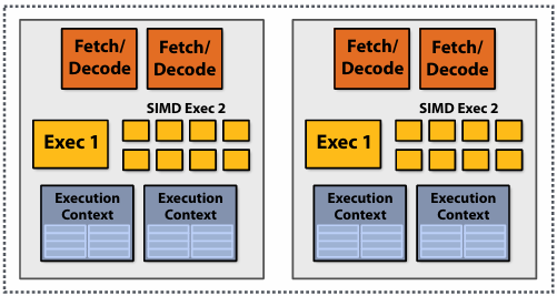
Lecture 2: A Modern Multi-Core Processor (Part I)
Key concepts about how modern parallel processors achieve high throughput(吞吐量)
Two concern(有关) parallel execution (multi-core, SIMD parallel execution)
One addresses(解决) the challenges of memory latency (multi-threading)
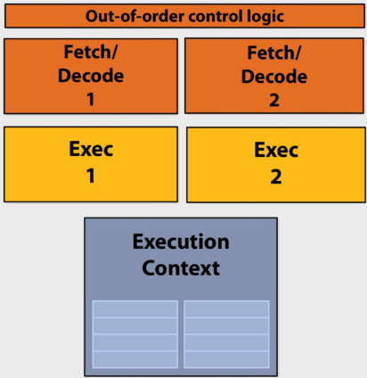
Pre multi-core era processor
Majority of chip transistors used to perform operations that help make a single instruction stream run fast
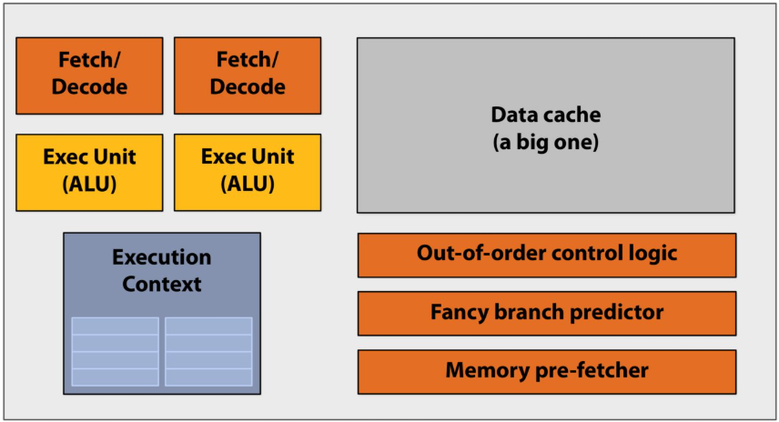
More transistors = larger cache, smarter out-of-order logic, smarter branch predictor, etc
Out-of-order control logic(乱序执行控制逻辑):打破指令在程序中原本的先后顺序,寻找可以并行执行的机会
Multi-core era processor
Use increasing transistor count to add more cores to the processor
SIMD processing(Single instruction, multiple data)
Add execution units(ALUs) to increase compute capability
Amortize(分摊) cost/complexity of managing an instruction stream across many ALUs
Same instruction broadcast to all ALUs
This operation is executed in parallel on all ALUs
Mask (discard) output of ALU
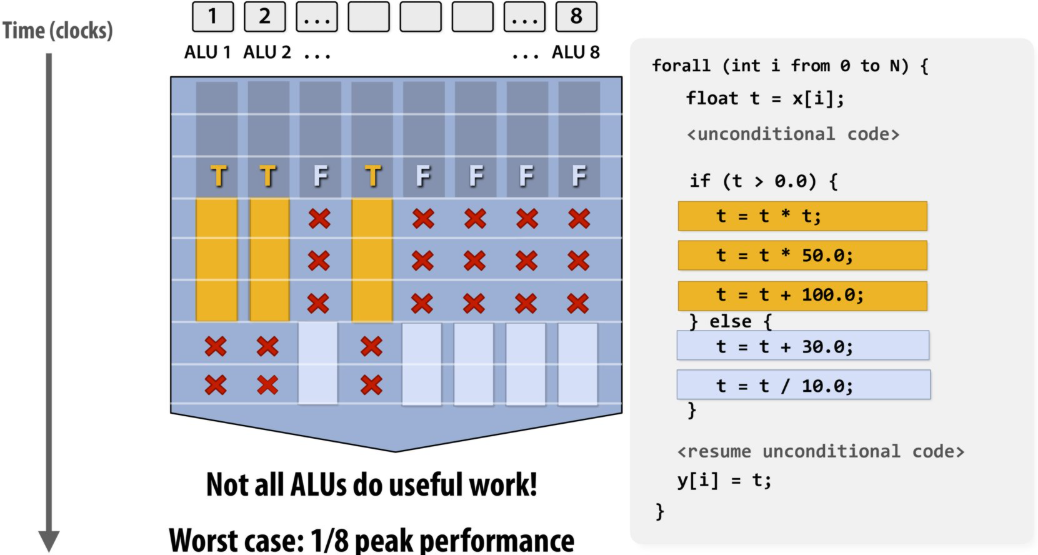
The program’s use of “forall” declares to the compiler that loop iterations are independent, and that same loop body will be executed on a large number of data elements
This abstraction can facilitate(促进) automatic generation of both multi-core parallel code, and vector instructions to make use of SIMD processing capabilities within a core
当代码运行到 if (t > 0.0) 时,如果 8 个通道里的数据,有些满足条件(T),有些不满足(F),硬件无法让一部分 ALU 跑 if 里的代码,另一部分跑 else 里的
硬件的处理方式是:
第一步: 掩码(Masking)掉所有 F 的通道,只让 T 的通道执行 if 分支里的代码。此时,F 对应的 ALU 是闲置的(如你图中带红色叉号 X 的部分)
第二步: 掩码掉所有 T 的通道,再让 F 的通道执行 else 分支里的代码。此时,T 对应的 ALU 是闲置的
结果: 总耗时 = 执行 if 分支的时间 + 执行 else 分支的时间。原本并行的 8 个核心,在这一刻退化成了类似于串行的工作方式,吞吐量大幅下降
如果所有元素全都在同一个分支里(比如全是正数),处理器就只需要花执行 A 的时间,效率会提高一倍
Some common jargon(术语)
Instruction stream coherence(一致性)(“coherent execution”)
Property(特性) of a program where the same instruction sequence applies to many data elements
Coherent execution IS NECESSARY for SIMD processing resources to be used efficiently
Coherent execution IS NOT NECESSARY for efficient parallelization across different cores, since each core has the capability to fetch/decode a different instructions from their thread’s instruction stream
“Divergent(发散)” execution
A lack of instruction stream coherence in a program
Instruction are generated by the compiler
Parallelism explicitly requested by programmer using intrinsics(内部函数)
Parallelism conveyed using parallel language semantics(语义)(e.g., forall example)
Parallelism inferred by dependency analysis of loops by “auto-vectorizing” compiler
Terminology(术语): “explicit SIMD”: SIMD parallelization is performed at compile time
Can inspect program binary and see SIMD instructions (vstoreps, vmulps, etc.)
“Implicit SIMD”
Compiler generates a binary with scalar instructions
But N instances of the program are always run together on the processor
Hardware(not compiler) is responsible for simultaneously executing the same instruction from multiple program instances on different data on SIMD ALUs
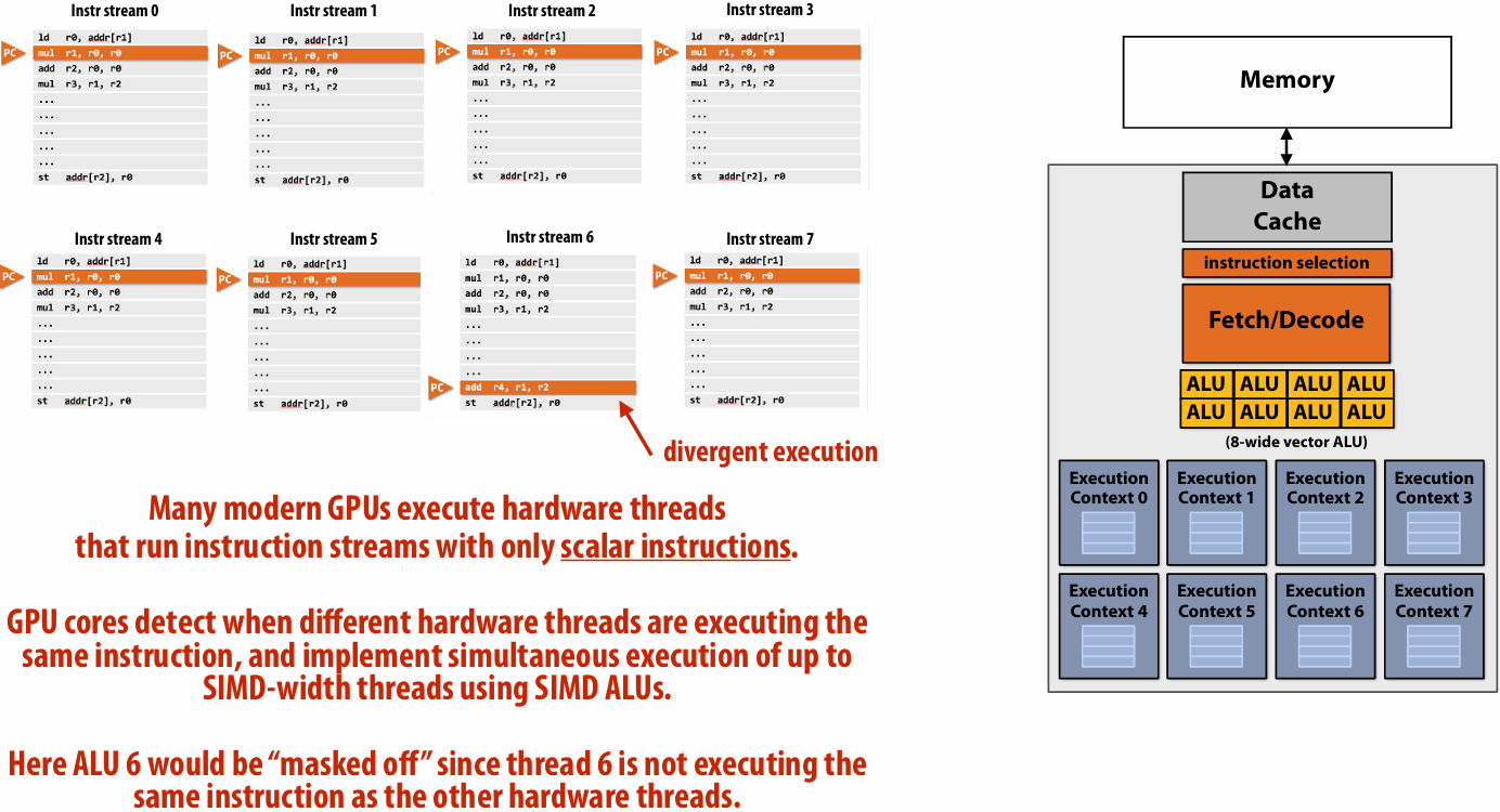
SIMD width of most modern GPUs ranges from 8 to 32
Divergent execution can be a big issue(poorly written code might execute at 1/32 the peak capability of the machine!)
Summary: three different forms of parallel execution
Superscalar: exploit ILP within an instruction stream. Process different instructions from the same instruction stream in parallel(within a core)
SIMD: multiple ALUs controlled by same instruction(within a core)
Efficient for data-parallel workloads: amortize control costs over many ALUs
Vectorization(向量化) done by compiler (explicit SIMD) or at runtime by hardware(implicit SIMD)
Multi-core: use multiple processing cores
Provides thread-level parallelism: simultaneously execute a completely different instruction stream on each core
Software creates threads to expose parallelism to hardware(e.g., via threading API)
Hardware-supported multi-threading
Data prefetching(预取) reduces stalls (hides latency)
Many modern CPUs have logic for guessing what data will be accessed in the future and “pre-fetching” this data into caches
Dynamically analyze program’s memory access patterns to make predictions
Prefetching reduces stalls since data is resident in cache when accessed
Note: Prefetching can also reduce performance if the guess is wrong(consumes bandwidth, pollutes caches)
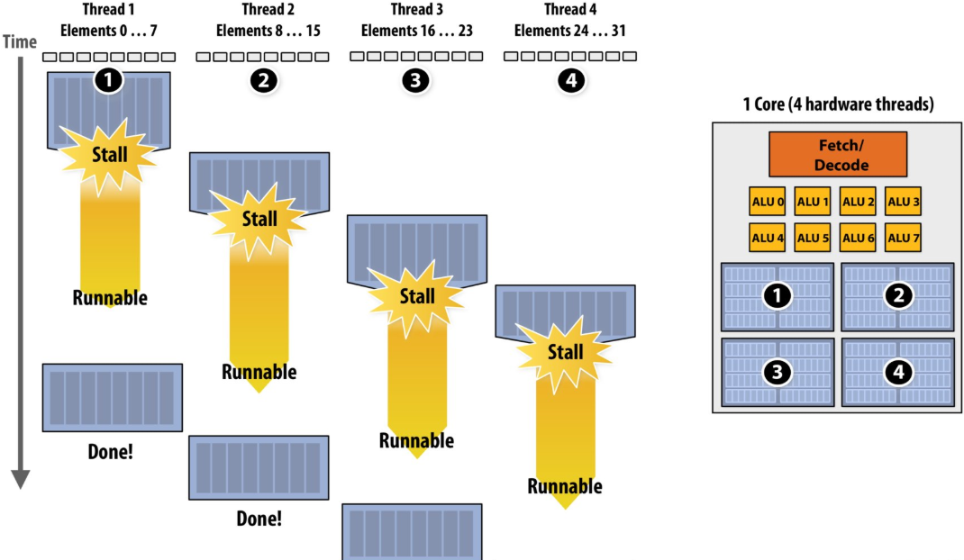
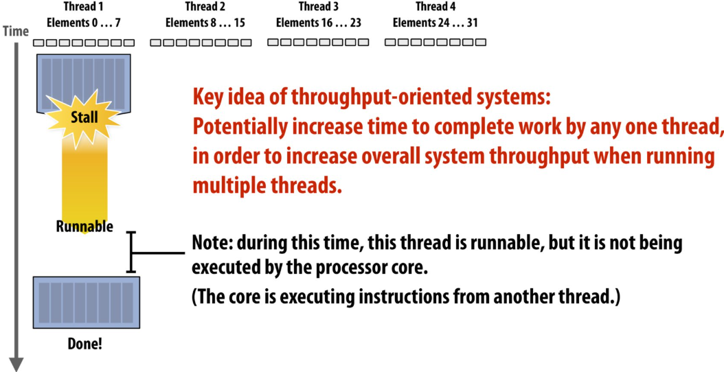
Multi-threading reduces stalls
interleave(交错) processing of multiple threads on the same core to hide stalls
if you can’t make progress on the current thread… work on another one
Hiding stalls with multi-threading
Throughput(吞吐量) computing: a trade-off(权衡)
No free lunch: storing execution contexts
Consider on-chip storage of execution contexts as a finite resource
Many small contexts (high latency hiding ability)
16 hardware threads: storage for small working set per thread
Four large contexts (low latency hiding ability)
4 hardware threads: storage for large working set per thread
Takeaway (point 1):
A processor with multiple hardware threads has the ability to avoid stalls by performing instructions from other threads when one thread must wait for a long latency operation to complete
Note: the latency of the memory operation is not changed by multi threading, it just no longer causes reduced processor utilization
Takeaway (point 2):
A multi-threaded processor hides memory latency by performing arithmetic from other threads
Programs that feature more arithmetic per memory access need fewer threads to hide memory stalls
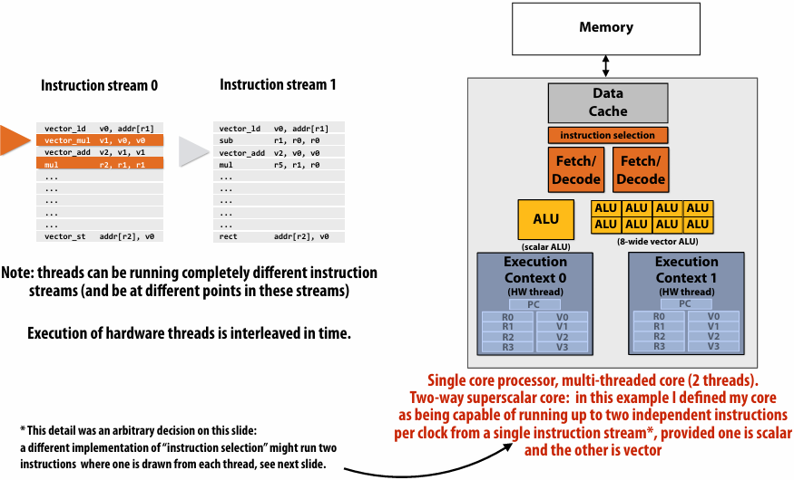
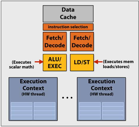
Hardware-supported multi-threading
- Core manages execution contexts for multiple threads
Core still has the same number of ALU resources: multi-threading only helps use them more efficiently in the face of high-latency operations like memory access
Processor makes decision about which thread to run each clock - Interleaved multi-threading (a.k.a.(又称) temporal multi-threading)
each clock, the core chooses a thread, and runs an instruction from the thread on the core’s ALUs - Simultaneous(同步) multi-threading (SMT)
Each clock, core chooses instructions from multiple threads to run on ALUs
Example: Intel Hyper-threading (2 threads per core)
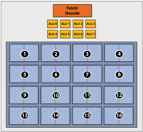
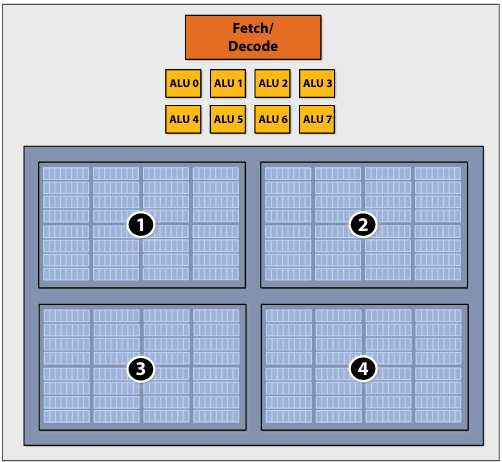
Kayvon’s fictitious(虚构) multi-core chip
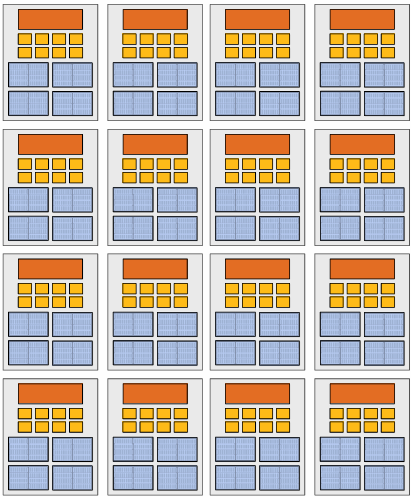
16 cores
8 SIMD ALUs per core (128 total)
4 threads per core
16 simultaneous instruction streams
64 total concurrent(同步) instruction streams
512 independent pieces of work are needed to run chip with maximal latency hiding ability
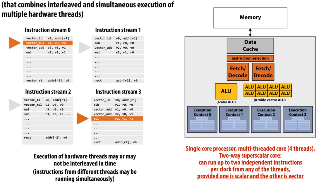
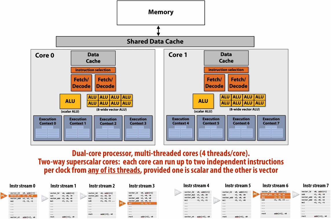
Example: Intel Skylake/Kaby Lake core
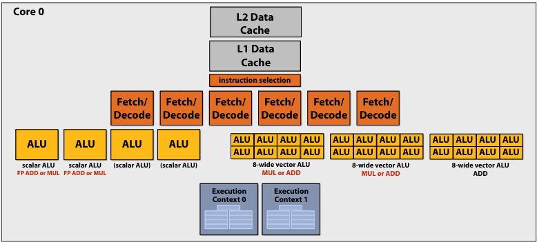
Two-way multi-threaded cores (2 threads)
Each core can run up to(最多) four independent scalar instructions
and up to three 8-wide vector instructions (up to 2 vector mul or 3 vector add)
GPUs: extreme throughput-oriented(面向吞吐量) processors
NVIDIA V100
There are 80 SM cores on the V100: That’s 163,840 pieces of data being processed concurrently to get maximal latency hiding!
The story so far…
To utilize modern parallel processors efficiently, an application must:
1.Have sufficient parallel work to utilize all available execution units (across many cores and many execution units per core)
2.Groups of parallel work items must require the same sequences of instructions (to utilize SIMD execution)
3.Expose more parallel work than processor ALUs to enable interleaving of work to hide memory stalls
Summary
Suggestion to students: know these terms
▪ Instruction stream
▪ Multi-core processor
▪ SIMD execution
▪ Coherent control flow(流)
▪ Hardware multi-threading
Interleaved multi-threading
Simultaneous multi-threading
Running code on a simple processor
Superscalar core
SIMD execution capability
Heterogeneous(异构) superscalar (scalar + SIMD)
Multi-threaded core
Multi-threaded, superscalar core
Multi-core, with multi-threaded, superscalar cores
Example: Intel Skylake/Kaby Lake core
Two-way multi-threaded cores (2 threads)
Each core can run up to(最多) four independent scalar instructions
and up to three 8-wide vector instructions (up to 2 vector mul or 3 vector add)
GPU “SIMT” (single instruction multiple thread)
Thought experiment
You write an application that spawns two threads
The application runs on the processor shown below
Two cores, two-execution contexts per core, up to instructions per clock, one instruction is an 8-wide SIMD instruction
Question: “who” is responsible for mapping the applications’s threads to the processor’s thread execution contexts?
Answer: the operating system
Question: If you were implementing the OS, how would to assign the two threads to the four execution contexts?
Answer: 优先分在不同的核心(Core)上,以避免资源争抢
例外情况: 两个线程之间有极其频繁的数据交换(需要共享 L1 Cache)
Another question: How would you assign threads to execution contexts if your C program spawned five threads?
Answer: 时分复用(Time-sharing)与负载均衡
Lecture 3: Modern Multi-Core Architecture (Part II) + ISPC Programming Abstractions
latency and bandwidth
Memory bandwidth
The rate at which the memory system can provide data to a processor
Example: 20 GB/s
Pipelining
Consider a program that runs threads that repeat the following sequence of three dependent instructions
1.X = load 64 bytes
2.Y = add x + x
3.Z = add x + y
Let’s say we’re running this sequence on many threads of a multi-threaded(Assume there are plenty of hardware threads to hide memory latency) core that:
Executes one math operation per clock
Can issue load instructions in parallel with math
Receives 8 bytes/clock from memory
Processor that can do one add per clock (+ co-issues(同时执行) LDs)
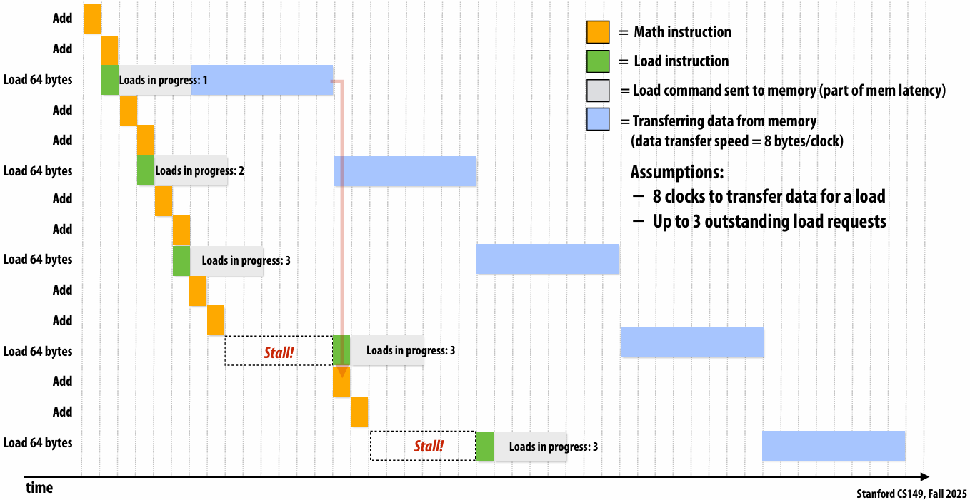
outstanding(未完成的)
Rate of completing math instructions is limited by memory bandwidth

bandwidth-bound(带宽受限)
High bandwidth memories
Modern GPUs leverage(利用) high bandwidth memories located near processor
Example:
V100 uses HBM2
900 GB/s
Computation is bandwidth limited!
If processors request data at too high a rate, the memory system cannot keep up
Overcoming bandwidth limits is often the most important challenge facing software developers targeting modern throughput-optimized(优化) systems
In modern computing, bandwidth is the critical resource
Performant parallel programs will:
Organize computation to fetch data from memory less often
Reuse data previously loaded by the same thread (temporal locality optimizations)
Share data across threads (inter-thread(线程间) cooperation)
Favor(优先) performing additional arithmetic(算术运算) to storing/reloading values (the math is “free”)
Main point: programs must access memory infrequently to utilize modern processors efficiently
Abstraction vs. implementation
Semantics(语义): what do the operations provided by a programming model mean?
Given a program, and given the semantics (meaning) of the operations used, what is the answer that the program will compute?
Implementation (aka scheduling(调度)): how will the answer be computed on a parallel machine?
In what (potentially parallel) order will be a program’s operations be executed?
Which operations will be computed by each thread?
Each execution unit? Each lane(通道) of a vector instruction?
Your goal as a student:
Given a program and knowledge of how a parallel programming model is implemented, in your head can you “trace” through what each part of the parallel computer is doing during each step of program
Programming with ISPC
Intel SPMD Program Compiler (ISPC)
SPMD: single program multiple data
ispc/ispc: Intel® Implicit SPMD Program Compiler
Intel® Implicit SPMD Program Compiler
A great read: “The Story of ISPC” (by Matt Pharr) : The story of ispc: all the links
example program
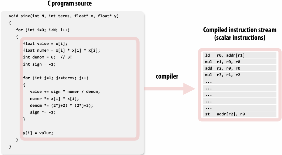
Compute sin(x) using Taylor expansion: sin(x) = x - x3/3! + x5/5! - x7/7! + …
for each element of an array of N floating-point numbers
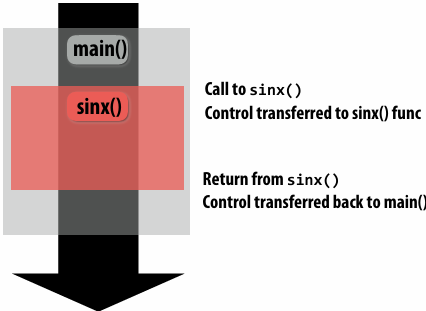
Invoking sinx()
1 | // C++ code: main.cpp |
1 | // C++ code: sinx.cpp |
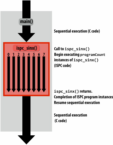
sinx() in ISPC
1 | // C++ code: main.cpp |
1 | // ISPC code: sinx.ispc |
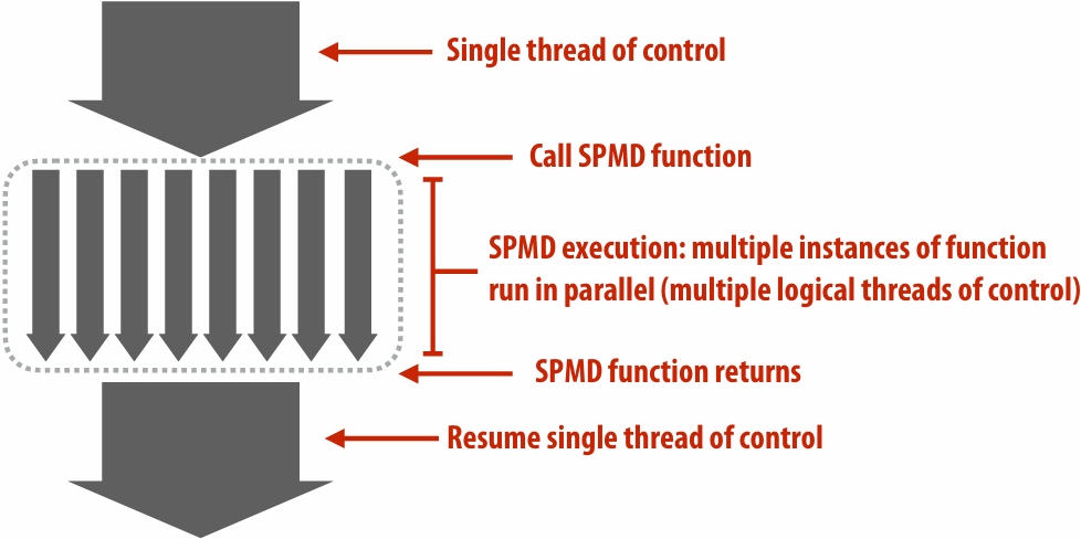
SPMD programming abstraction:
Call to ISPC function spawns “gang(组)” of ISPC “program instances”
All instances run ISPC code concurrently
Each instance has its own copy of local variables( programIndex int float )
Upon return, all instances have completed
ISPC language keywords:
programCount: number of simultaneously executing instances in the gang (uniform value)
programIndex: id of the current instance in the gang. (a non-uniform value: “varying”)
uniform: A type modifier. All instances have the same value for this variable. Its use is purely an optimization. Not needed for correctness
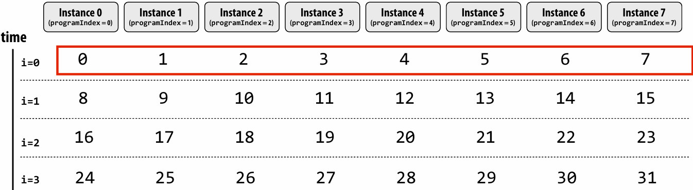
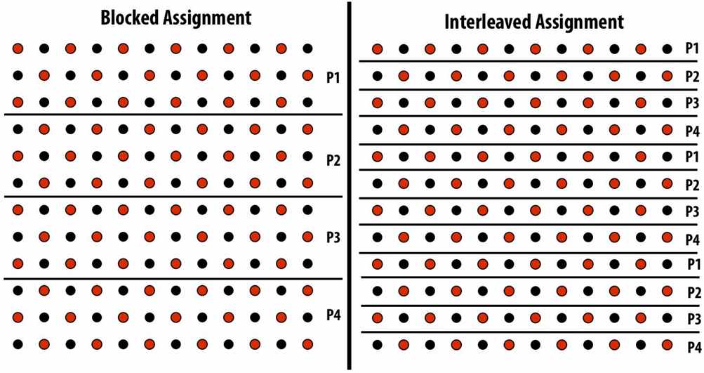
“Interleaved” assignment of array elements to program instances
Invoking sinx() in ISPC
In this illustration programCount = 8
Interleaved assignment of program instances to loop iterations
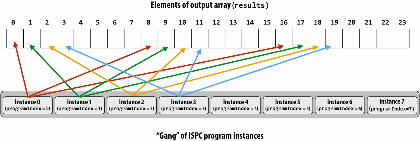
In this illustration: gang contains eight instances: programCount = 8
ISPC implements the gang abstraction using SIMD instructions
ISPC compiler generates SIMD implementation:
Number of instances in a gang is the SIMD width of the hardware (or a small multiple of SIMD width)
ISPC compiler generates a C++ function binary (.o) whose body contains SIMD instructions
C++ code links against generated object file as usual
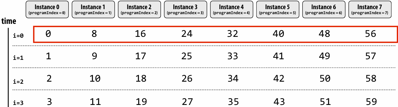
sinx() in ISPC: version 2
“Blocked” assignment of array elements to program instances
1 | // C++ code: main.cpp |
1 | // ISPC code: sinx.ispc |
Blocked assignment of program instances to loop iterations
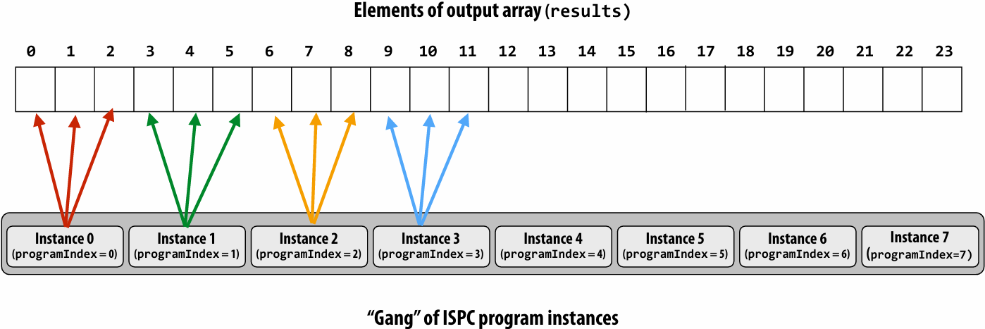
In this illustration: gang contains eight instances: programCount = 8
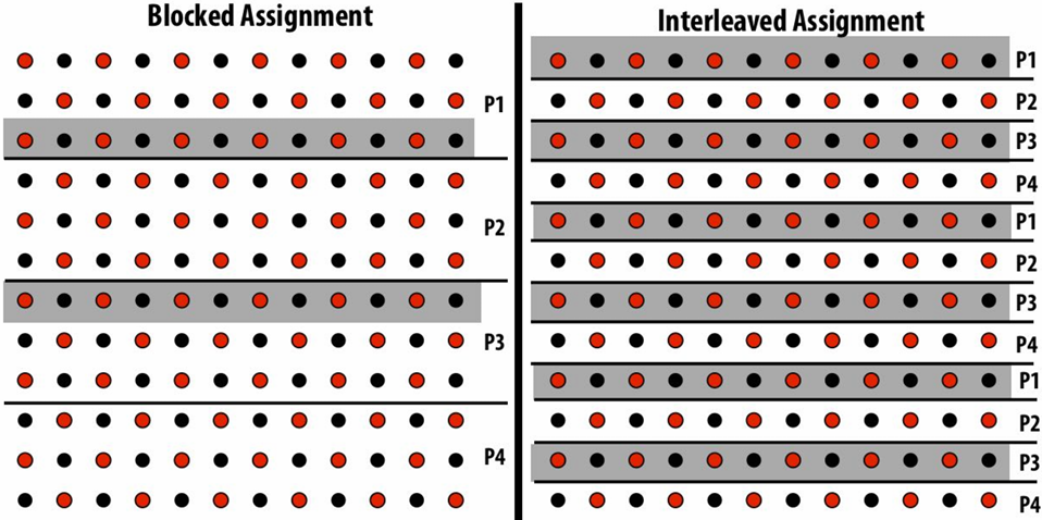
Schedule: interleaved assignment
“Gang” of ISPC program instances
Gang contains four instances: programCount = 8
A single “packed vector load” instruction (vmovaps (see _mm256_load_ps() intrinsic function) ) efficiently implements:
float value = x[idx];
for all program instances, since the eight values are contiguous in memory
Schedule: blocked assignment
“Gang” of ISPC program instances
Gang contains four instances: programCount = 8
float value = x[idx];
For all program instances now touches eight non-contiguous values in memory
Need “gather” instruction (vgatherdps (see _mm256_i32gather_ps() intrinsic function) ) to implement (gather is a more complex, and more costly SIMD instruction…)
Raising level of abstraction with foreach
1 | // C++ code: main.cpp |
1 | // ISPC code: sinx.ispc |
foreach: key ISPC language construct
foreach declares parallel loop iterations
Programmer says: these are the iterations the entire gang (not each instance) must perform
ISPC implementation takes responsibility for assigning iterations to program instances in the gang
How might foreach be implemented?
Code written using foreach abstraction:
1 | foreach (i = 0 ... N) |
Implementation 1: program instance 0 executes all iterations
1 | if (programCount == 0) { |
Implementation 2: interleave iterations onto program instances
1 | // assume N % programCount = 0 |
Implementation 3: block iterations onto program instances
1 | // assume N % programCount = 0 |
Implementation 4: dynamic assignment of iterations to instances
1 | uniform int nextIter; |
Thinking about iterations, not parallel execution
In many simple cases, using foreach allows the programmer to express their program almost as if it was a sequential program
1 | export void ispc_function( |
What does this program do?
1 | // main C++ code: |
1 | // ISPC code: |
This ISPC program computes the absolute value of elements of x, then repeats it twice in the output array y
1 | // main C++ code: |
1 | // ISPC code: |
The output of this program is undefined!
Possible for multiple iterations of the loop body to write to same memory location
Computing the sum of all elements in an array (incorrectly)
What’s the error in this program?
1 | export uniform float sum_incorrect_1( |
sum is of type float (different variable for all program instances)
Cannot return many copies of a varianble to the calling C code, which expects one return value of type float
Result: compile-time type error
What’s the error in this program?
1 | export uniform float sum_incorrect_2( |
sum is of type uniform float (one copy of variable for all program instances)
x[i] has a different value for each program instance
So what gets copied into sum? (一份sum,多份x[i],无法让多个并行的实例同时修改同一个变量)
Result: compile-time type error
Computing the sum of all elements in an array (correctly)
1 | export uniform float sum_array( |
Each instance accumulates a private partial sum (no communication)
Partial sums are added together using the reduce_add() cross-instance communication primitive
The result is the same total sum for all program instances (reduce_add() returns a uniform float)
The ISPC code will execute in a manner similar to the C code with AVX intrinsics implemented below
1 | float sum_summary_AVX(int N, float* x) { |
ISPC’s cross program instance operations
Compute sum of a variable’s value in all program instances in a gang:
1 | uniform int64 reduce_add(int32 x); |
Compute the min of all values in a gang:
1 | uniform int32 reduce_min(int32 a); |
Broadcast a value from one instance to all instances in a gang:
1 | int32 broadcast(int32 value, uniform int index); |
For all i, pass value from instance i to the instance i+offset % programCount:
1 | int32 rotate(int32 value, uniform int offset); |
ISPC: abstraction vs. implementation
Single program, multiple data (SPMD) programming model
Programmer “thinks”: running a gang is spawning programCount logical instruction streams (each with a different value of programIndex)
This is the programming abstraction
Program is written in terms of this abstractionSingle instruction, multiple data (SIMD) implementation
ISPC compiler emits vector instructions (e.g., AVX2, ARM NEON) that carry out the logic performed by a ISPC gang
ISPC compiler handles mapping of conditional control flow to vector instructions (by masking vector lanes, etc. like you do manually in assignment 1)Semantics of ISPC can be tricky(棘手的)
SPMD abstraction + uniform values (allows implementation details to peek through(透过) abstraction a bit)
SPMD programming model summary
SPMD = “single program, multiple data”
Define one function, run multiple instances of that function in parallel on different input arguments
ISPC tasks
- The ISPC gang abstraction is implemented by SIMD instructions that execute within on thread running on one x86 core of a CPU
- So all the code I’ve shown you in the previous slides would have executed on only one of the four cores of the myth machines(斯坦福大学计算机科学系(Stanford CS)提供的专供学生使用的公共 Linux 计算集群)
- ISPC contains another abstraction: a “task” that is used to achieve multi-core execution. I’ll let you read up about that as you do assignment 1
An ISPC task is just a task. A thread would be an implementation detail. But it’s very true that if you create eight tasks, a smart thing for ISPC to do would be under the hood, spawn eight threads and run them all on different threads. But if you create 100,000 tasks, it probably would be pretty dumb for ISPC to create 100,000 threads.
How does a computer that needs to run apparently a 700 kernel threads right now, how does it run 700 kernel threads on computer?
It’s got a context switch
The operating system from time t o time is saying, here are those eight threads that need to run. I’m going to put them on the processor and let the processor run. And periodically, some timer expires, and the operating system says, well, we have 700 threads. We need to have another 8 run. So we’re going to rip those threads off the processor and put those on. And you can imagine that could be pretty slow
operating system context switch vs. hardware execution context switch
| 特性 | 硬件多线程 (Hardware Multi-threading) | 操作系统上下文切换 (OS Context Switch) |
|---|---|---|
| 谁来做 | 硬件(电路) 自动完成 | 软件(内核代码) 执行指令完成 |
| 寄存器 | 复制多份(每个线程有独立的物理寄存器组) | 只有一套(切换时必须把内容存到 RAM) |
| 切换耗时 | 极快(通常 0 - 数个周期) | 极慢(数千到数十万个周期) |
| 切换触发点 | 硬件检测到 Stall(如 Cache Miss) | 时间片到期、I/O 阻塞、系统调用 |
| 主要目标 | 延迟隐藏 (Latency Hiding),榨干执行单元 | 任务管理、公平性、多任务并发 |
ISPC is a low-level programming language: by exposing(公开) programIndex and programCount, it allows programmer to define what work each program instance does and what data each instance accesses
Can implement programs with undefined output
Can implement programs that are correct only for a specific programCount
Everything outside a foreach must be uniform values and uniform logic(确保程序的控制流在进入并行区域前是明确且同步的)
串行上下文与并行上下文的切换:在 ISPC 中,代码的运行逻辑可以看作是“单线程入口,局部并行”
Outside foreach(外部):代码处于串行控制流中。此时,编译器认为它是在为“整组”程序实例(整个 SIMD 单元)做决策。既然是为整组做决策,所有的变量值和逻辑判断就必须对所有实例都一致(即 uniform)
Inside foreach(内部):这是并行开始的地方。foreach 负责把数据分配给不同的程序实例(Program Instances)。只有在这里,变量才可以是 varying 的(每个实例拥有不同的值)
硬件效率与寄存器利用
uniform 变量:通常存储在 CPU 的标量寄存器(Scalar Registers)中。它们只占一份空间,计算速度极快
varying 变量:存储在 SIMD 向量寄存器中
如果外部变量都是 uniform 的,编译器可以进行大量的优化,避免不必要的向量运算,减少内存带宽压力。只有在真正处理大量数组元素(foreach 内部)时,才动用沉重的向量资源
Summary
Programming models provide a way to think about the organization of parallel programs
They provide abstractions that permit multiple valid implementations
I want you to always be thinking about abstraction vs. implementation for the remainder(剩余部分) of this course
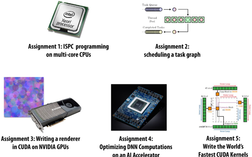
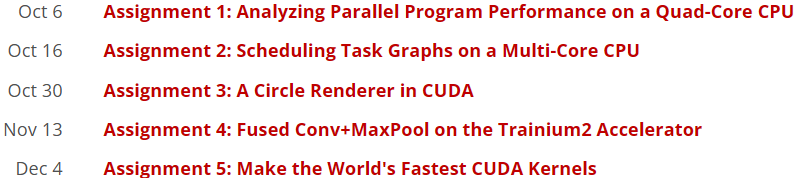
Assignment 1: Analyzing Parallel Program Performance on a Quad-Core CPU
搭建本地Linux开发环境
安装WSL2(Windows Subsystem for Linux)
1.以管理员权限打开PowerShell,运行: wsl –install
2.在Microsoft Store下载 Ubuntu 22.04 LTS
3.优点:你可以在Ubuntu里写C++/CUDA 代码,但依然能用Windows的浏览器看视频、查文档
Windows 安装 WSL2 并运行 Ubuntu 22.04 指南本文为 Windows 10 和 Windows - 掘金
安装 WSL | Microsoft Learn
如果显示正在安装: Ubuntu 这时候卡住在0%(微软商店抽风),那么我们执行如下指令,从GitHub下载
1 | wsl --install -d Ubuntu --web-download |
配置 CUDA Toolkit
1.在 Windows主机安装最新的NVIDIA 驱动
2.在 WSL2(Ubuntu)里安装 CUDA Toolkit(注意要选Linux-WSL 版本)
3.安装完成后,输入nvcc -V, 看到版本号即表示成功
WLS2安装CUDA保姆级教程_wsl2 cuda-CSDN博客
IDE选择
使用Vs Code,并安装”Remote - WSL”扩展
这样你可以在 Windows界面操作,但所有的编译和运行都在WSL2的Linux环境下进行
开始将 VS Code 与 WSL 配合使用 | Microsoft Learn
Using C++ and WSL in VS Code
具体内容和实现
[WorldClass/Stanford CS149 Parallel Computing/asst1 at master · tiny-star3/WorldClass](https://github.com/tiny-star3/WorldClass/tree/master/Stanford CS149 Parallel Computing/asst1)
Lecture 4: Parallelizing Code: The Programming Thought Process
Creating a parallel program
Your thought process:
Identify work that can be performed in parallel
Partition work (and also data associated with the work)
Manage data access, communication, and synchronization
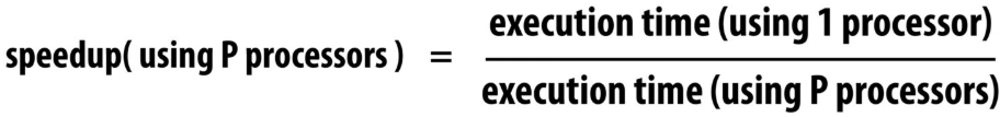
A common goal is maximizing speedup
For a fixed computation: Speedup(P processors) = Time(1 processor) / Time (P processors)
Other goals include achieving high efficiency (cost, area, power, etc.) or working on bigger problems than can fit on one machine
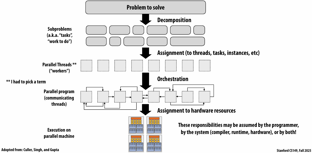
Orchestration 编排
Problem decomposition
Break up problem into tasks that can be carried out in parallel
In general: create at least enough tasks to keep all execution units on a machine busy
Key challenge of decomposition: identifying dependencies (or… a lack of dependencies)
Amdahl’s Law: dependencies limit maximum speedup due to parallelism
Let S = the fraction(比例) of sequential execution that is inherently sequential (dependencies prevent parallel execution)
Then maximum speedup due to parallel execution ≤ 1/S
Max speedup on P processors given by:
Assignment
Assigning tasks to workers
Think of “tasks” as things to do
What are “workers”? (Might be threads, program instances, vector lanes, etc.)
Goals: achieve good workload balance, reduce communication costs
Can be performed statically (before application is run), or dynamically as program executes
Although programmer is often responsible for decomposition, many languages/runtimes take responsibility for assignment
static assignment using C++11 threads
Dynamic assignment using ISPC tasks
Orchestration
Involves:
Structuring communication
Adding synchronization to preserve(维持) dependencies if necessary
Organizing data structures in memory
Scheduling tasks
Goals: reduce costs of communication/sync, preserve locality of data reference, reduce overhead, etc.
Machine details impact many of these decisions
If synchronization is expensive, programmer might use it more sparsely(少)
Assignment to hardware
Assign “threads” (“workers”) to hardware execution units
Example 1: assignment to hardware by the operating system
e.g., map a thread to HW execution context on a CPU core
Example 2: assignment to hardware by the compiler
e.g., Map ISPC program instances to vector instruction lanes
Example 3: assignment to hardware by the hardware
e.g., Map CUDA thread blocks to GPU cores (discussed in a future lecture)
Many interesting decisions:
Place related threads (cooperating threads) on the same core (maximize locality, data sharing, minimize costs of comm/sync)
Place unrelated threads on the same core (one might be bandwidth limited and another might be compute limited) to use machine more efficiently
A parallel programming example
A 2D-grid based solver
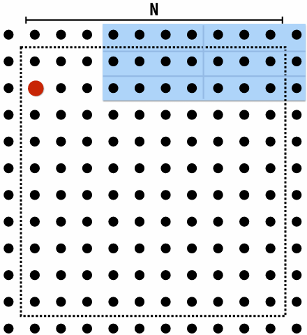
Problem: solve partial differential equation(偏微分方程) (PDE) on (N+2) x (N+2) grid
Solution uses iterative algorithm:
Perform Gauss-Seidel sweeps(高斯-赛德尔扫描) over grid until convergence
A[i,j] = 0.2 * (A[i,j] + A[i,j-1] + A[i-1,j] + A[i,j+1] + A[i+1,j]);

Grid solver algorithm: find the dependencies
Pseudocode for sequential algorithm is provided below
1 | const int n; |
Step 1: identify dependencies (problem decomposition phase)
Each row element depends on element to left
Each row depends on previous row
Note: the dependencies illustrated on this slide are grid element data dependencies in one iteration of the solver (in one iteration of the “while not done” loop)
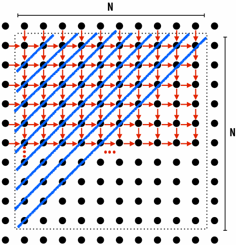
There is independent work along the diagonals!
Good: parallelism exists!
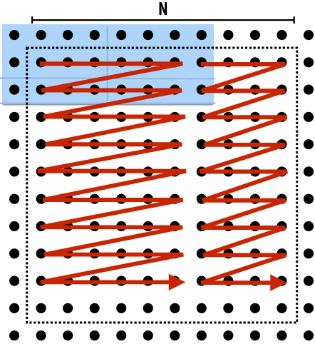
Possible implementation strategy:
1.Partition grid cells on a diagonal into tasks
2.Update values in parallel
3.When complete, move to next diagonal
Bad: independent work is hard to exploit
Not much parallelism at beginning and end of computation
Frequent synchronization (after completing each diagonal)
Idea: improve performance by changing the algorithm to one that is more amenable(适合) to parallelism
Change the order that grid cell cells are updated
New algorithm iterates to same solution (approximately), but converges to solution differently
Note: floating-point values computed are different, but solution still converges to within error threshold(误差阈值)
Yes, we needed domain knowledge of the Gauss-Seidel method to realize this change is permissible
This is a common technique in parallel programming
New approach: reorder grid cell update via red-black coloring
Reorder grid traversal(遍历顺序): red-black coloring
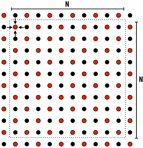
Update all red cells in parallel
When done updating red cells , update all black cells in parallel (respect dependency on red cells)
Repeat until convergence
Possible assignments of work to processors
Question: Which is better? Does it matter?
Answer: It depends on the system this program is running on
Consider dependencies in the program
1.Perform red cell update in parallel
2.Wait until all processors done with update
3.Communicate updated red cells to other processors
4.Perform black cell update in parallel
5.Wait until all processors done with update
6.Communicate updated black cells to other processors
7.Repeat
Communication resulting from assignment
shaded area = data that must be sent to P2 each iteration
Blocked assignment requires less data to be communicated between processors
Two ways to think about writing this program
Data parallel thinking
SPMD / shared address space
Data-parallel expression of grid solver
Note: to simplify pseudocode: just showing red-cell update
1 | const int n; |
Shared address space (with SPMD threads) expression of solver
Programmer is responsible for synchronization
Common synchronization primitives:
Locks (provide mutual exclusion): only one thread in the critical region at a time
Barriers: wait for threads to reach this point
1 | // Assume these are global variables (accessible to all threads) |
Synchronization in a shared address space
Shared address space model (abstraction)
Threads communicate by:
Reading/writing to shared variables in a shared address space(shared variables)
Communication between threads is implicit in memory loads/stores
Manipulating synchronization primitives(原语)
e.g., ensuring mutual exclusion via use of locks
This is a natural extension of sequential programming
Barrier synchronization primitivebarrier(num_threads)
Barriers are a conservative(保守) way to express dependencies
Barriers divide computation into phases
All computation by all threads before the barrier complete before any computation in any thread after the barrier begins
In other words, all computations after the barrier are assumed to depend on all computations before the barrier
Shared address space solver: one barrier
Idea: Remove dependencies by using different diff variables in successive(连续的) loop iterations
Trade off footprint(牺牲内存占用) for removing dependencies! (a common parallel programming technique)
1 | int n; |
Grid solver implementation in two programming models
Data-parallel programming model
Synchronization:
Single logical thread of control, but iterations of forall loop may be parallelized by the system (implicit barrier at end of forall loop body)
Communication
Implicit in loads and stores (like shared address space)
Special built-in primitives for more complex communication patterns: e.g., reduce
Shared address space
Synchronization:
Mutual exclusion required for shared variables (e.g., via locks)
Barriers used to express dependencies (between phases of computation)
Communication
Implicit in loads/stores to shared variables
Summary
Amdahl’s Law
Overall maximum speedup from parallelism is limited by amount of serial execution in a program
Aspects of creating a parallel program
Decomposition to create independent work, assignment of work to workers, orchestration (to coordinate(协调) processing of work by workers), mapping to hardware
We’ll talk a lot about making good decisions in each of these phases in the coming lectures
Focus today: identifying dependencies
Focus soon: identifying locality(局部性), reducing synchronization
Lecture 5: Performance Optimization Part 1: Work Distribution and Scheduling
Programming for high performance
Optimizing the performance of parallel programs is an iterative process of refining choices for decomposition, assignment, and orchestration…
Key goals (that are at odds with each other) (彼此冲突)
Balance workload onto available execution resources
Reduce communication (to avoid stalls)
Reduce extra work (overhead) performed to increase parallelism, manage assignment, reduce communication, etc
TIP #1: Always implement the simplest solution first, then measure performance to determine if you need to do better
Balancing the workload
Ideally: all processors are computing all the time during program execution
(they are computing simultaneously, and they finish their portion of the work at the same time)
Static assignment
Assignment of work to threads does not depend on dynamic behavior
Assignment not necessarily set at compile-time (we call it static is the assignment is determined when the amount of work and number of workers is known: assignment may depend on runtime parameters such as input data size, number of threads, etc.)
Good aspects of static assignment: simple, essentially zero runtime overhead to perform assignment
When is static assignment applicable?
When the cost (execution time) of work and the amount of work is predictable, allowing the programmer to work out a good assignment in advance
Simplest example: it is known up front that all work has the same cost
When work is predictable, but not all jobs have same cost
Jobs have unequal, but known cost: assign equal number of tasks to processors to ensure good load balance (on average)
When statistics about execution time are predictable (e.g., same cost on average)
“Semi-static” assignment
Cost of work is predictable for near-term future
Idea: recent past is a good predictor of near future
Application periodically(定期) profiles(分析) its execution and re-adjusts assignment
Assignment is “static” for the interval between re-adjustments
Dynamic assignment
Program determines assignment dynamically at runtime to ensure a well-distributed load
(The execution time of tasks, or the total number of tasks, is unknown or unpredictable.)
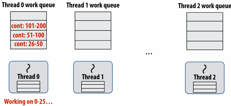
Dynamic assignment using a work queue
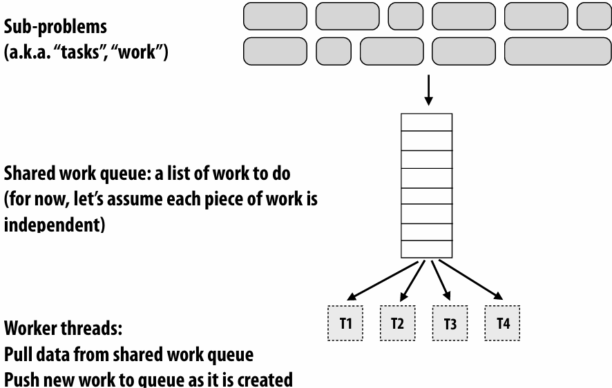
Choosing task size
Useful to have many more tasks than processors(many small tasks enables good workload balance via dynamic assignment)
Motivates small granularity tasks
But want as few tasks as possible to minimize overhead of managing the assignment
Motivates large granularity tasks
Ideal granularity depends on many factors(Common theme in this course: must know your workload, and your machine)
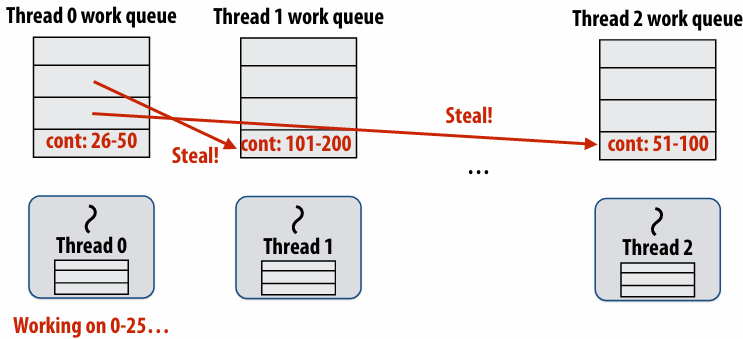
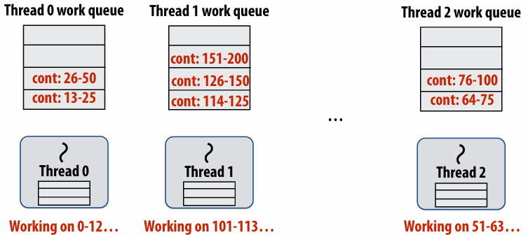
Decreasing synchronization overhead using distributed queues(avoid need for all workers to synchronize on single work queue)
Work in task queues need not be independent
Summary
Challenge: achieving good workload balance
Want all processors working all the time (otherwise(否则), resources are idle(空闲)!)
But want low-cost solution for achieving this balance
Minimize computational overhead (e.g., scheduling/assignment logic)
Minimize synchronization costs
Static assignment vs. dynamic assignment
Really, it is not an either/or(非此即彼) decision, there’s a continuum of choices
Use up-front(预先) knowledge about workload as much as possible to reduce load imbalance and task management/ synchronization costs (in the limit, if the system knows everything, use fully static assignment)
Scheduling fork-join parallelism
Common parallel programming patterns
Data parallelism:
Perform same sequence of operations on many data elements
Explicit management of parallelism with threads:
Create one thread per execution unit (or per amount of desired concurrency)
Consider divide-and-conquer algorithms
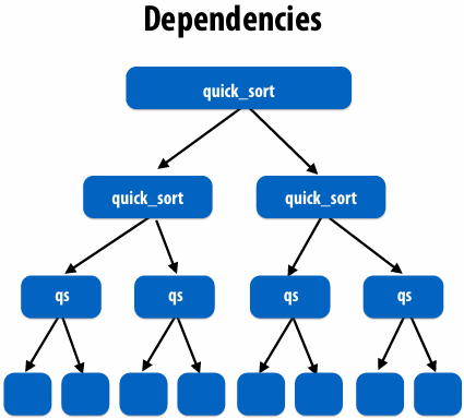
Quick sort:
1 | // sort elements from ‘begin’ up to (but not including) ‘end’ |
Fork-join pattern
Natural way to express the independent work that is inherent in divide-and-conquer algorithms
This lecture’s code examples will be in Cilk Plus
C++ language extension
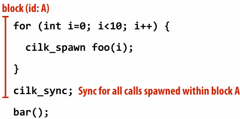
Originally developed at MIT, now adapted as open standard (in GCC, Intel ICC)cilk_spawn foo(args);
“fork” (create new logical thread of control)
Semantics: invoke foo, but unlike standard function call, caller may continue executing asynchronously with execution of foocilk_sync;
“join”
Semantics: returns when all calls spawned by current function have completed. (“sync up” with the spawned calls)
Note: there is an implicit cilk_sync at the end of every function that contains a cilk_spawn
(implication: when a Cilk function returns, all work associated with that function is complete)
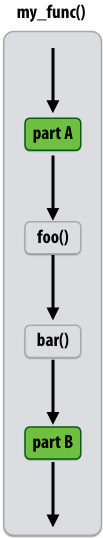
Call-return of a function in C(And many other languages)
1 | void my_func() { |
Semantics of a function call: Control moves to the function that is called (Thread executes instructions for the function)
When function returns, control returns back to caller (thread resumes(恢复) executing instructions from the caller)
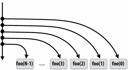
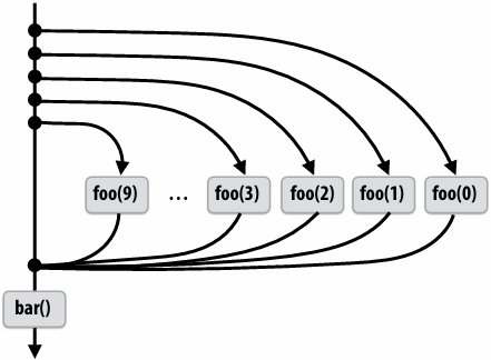
Basic Cilk Plus examples
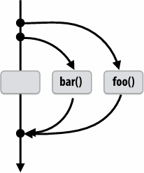
1 | // foo() and bar() may run in parallel |
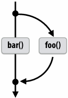
1 | // foo() and bar() may run in parallel |
Same amount of independent work first example, but potentially higher runtime overhead (due to two spawns vs. one)
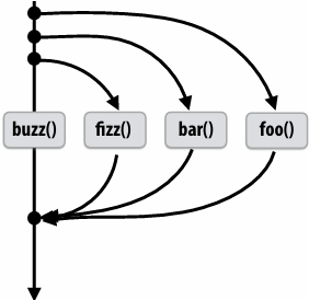
1 | // foo, bar, fizz, buzz, may run in parallel |
Abstraction vs. implementation
Notice that the cilk_spawn abstraction does not specify how or when spawned calls are scheduled to execute
Only that they may be run concurrently with caller (and with all other calls spawned by the caller)
An implementation of Cilk is correct if it implements cilk_spawn foo() the same way as it implementation a normal function call to foo()
But cilk_sync does serve as a constraint on scheduling
All spawned calls must complete before cilk_sync returns
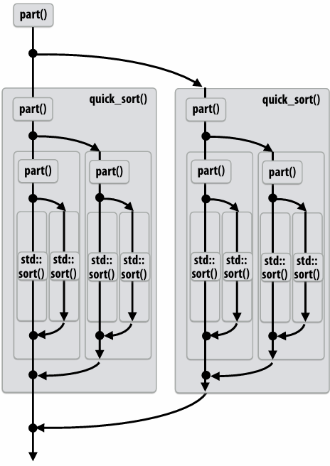
Parallel quicksort in Cilk Plus
1 | void quick_sort(int* begin, int* end){ |
Writing fork-join programs
Main idea: expose independent work (potential parallelism) to the system using cilk_spawn
Recall parallel programming rules of thumb
Want at least as much work as parallel execution capability (e.g., program should probably spawn at least as much work as needed to fill all the machine’s processing resources)
Want more independent work than execution capability to allow for good workload balance of all the work onto the cores
“parallel slack” = ratio of independent work to machine’s parallel execution capability (in practice: ~8 is a good ratio)
But not too much independent work so that granularity of work is too small (too much slack incurs overhead of managing fine-grained(细粒度) work)
Scheduling fork-join programs
Consider very simple scheduler:
Launch pthread for each cilk_spawn using pthread_create
Translate cilk_sync into appropriate pthread_join calls
Potential performance problems?
Heavyweight spawn operation
Many more concurrently running threads than cores
Context switching overhead
Larger working set than necessary, less cache locality
Note: now we are going to talk about the implementation of Cilk
Pool of worker threads
The Cilk Plus runtime maintains pool of worker threads
Think: all threads are created at application launch(It’s perfectly fine to think about it this way, but in reality, runtimes tend to be lazy and initialize worker threads on the first Cilk spawn. (This is a common implementation strategy, ISPC does the same with worker threads that run ISPC tasks.))
Exactly as many worker threads as execution contexts in the machine
Consider execution of the following code
1 | // spawned child |
Specifically, consider execution from the point foo() is spawned
First, consider a serial implementation
Run child first… via a regular function call
Thread runs foo(), then returns from foo(), then runs bar()
Continuation is implicit in the thread’s stack
Per-thread work queues store “work to do”
Upon reaching cilk_spawn foo(), thread places continuation in its work queue, and begins executing foo()
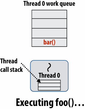

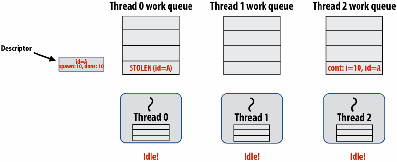
Idle threads “steal” work from busy threads
If thread 1 goes idle (a.k.a. there is no work in its own queue), then it looks in thread 0’s queue for work to do
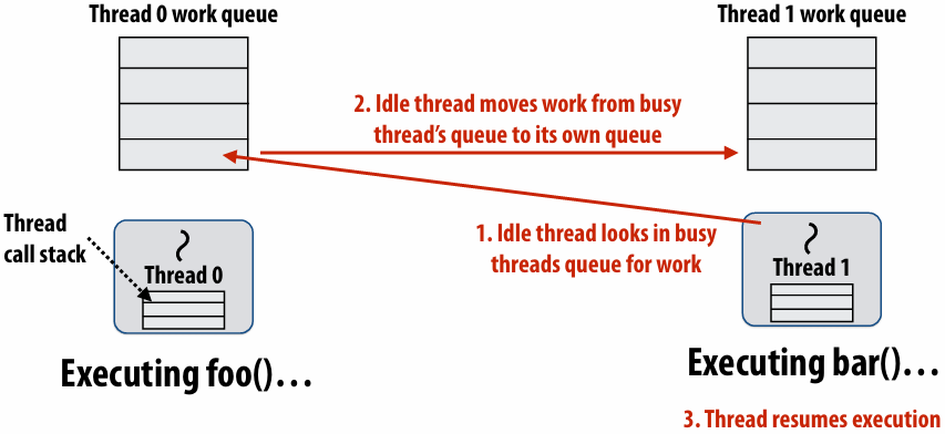
Run continuation first: queue child for later execution
Child is made available for stealing by other threads (“child stealing”)
Run child first: enqueue continuation for later execution
Continuation is made available for stealing by other threads (“continuation stealing”)
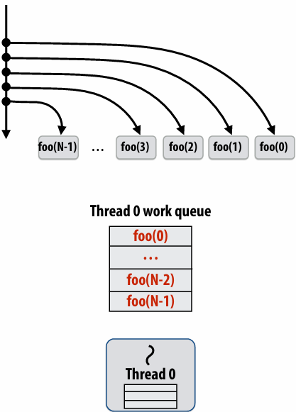
Run continuation first (“child stealing”)
Caller thread spawns work for all iterations before executing any of it
Think: breadth-first traversal(广度优先遍历) of call graph. O(N) space for spawned work (maximum space)
If no stealing, execution order is very different than that of program with cilk_spawn removed
Run child first (“continuation stealing”)
Caller thread only creates one item to steal (continuation that represents all remaining iterations)
If no stealing occurs, thread continually pops continuation from work queue, enqueues new continuation (with updated value of i)
Order of execution is the same as for program with spawn removed
Think: depth-first traversal(深度优先遍历) of call graph
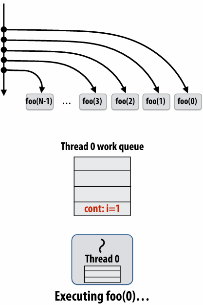
Enqueues continuation with i advanced by 1
If continuation is stolen, stealing thread spawns and executes next iteration
Can prove that work queue storage for system with T threads is no more than T times that of stack storage for single threaded execution
Scheduling quicksort: assume 200 elements
1 | void quick_sort(int* begin, int* end) { |
Implementing work stealing: dequeue per worker
Work queue implemented as a dequeue (double ended queue)
Local thread pushes/pops from the “tail” (bottom)
Remote threads steal from “head” (top)
Implementing work stealing: choice of victim
Idle threads randomly choose a thread to attempt to steal from
Steal work from top of dequeue:
Steals largest amount of work (reduce number of steals)
Maximum locality in work each thread performs (when combined with run child first scheme)
Stealing thread and local thread do not contend(争用) for same elements of dequeue(efficient lock-free implementations of dequeue exist)
Child-first work stealing scheduler anticipates divide-and-conquer parallelism
1 | for (int i=0; i<N; i++) { |
1 | void recursive_for(int start, int end) { |
Code at second generates work in parallel, (code at first does not), so it more quickly fills up parallel machine
Implementing sync
Implementing sync: no stealing case
If no work has been stolen by other threads, then there’s nothing to do at the sync point
cilk_sync is a no-op
Implementing sync: stealing case
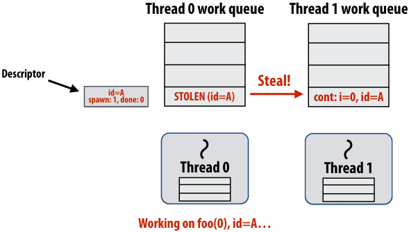
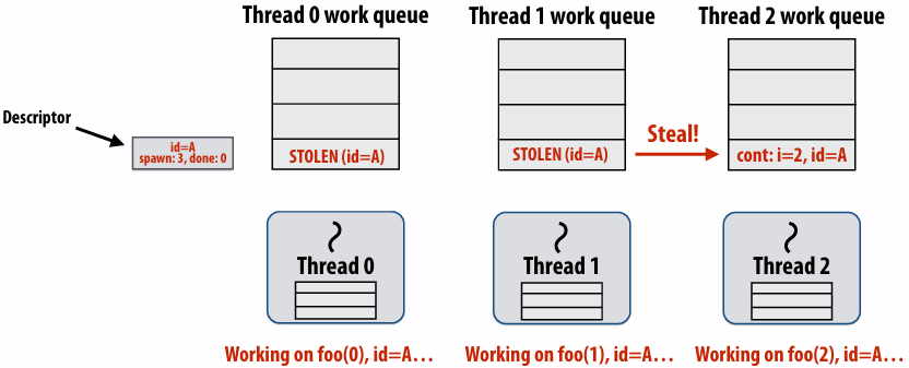
Idle thread 1 steals from busy thread 0
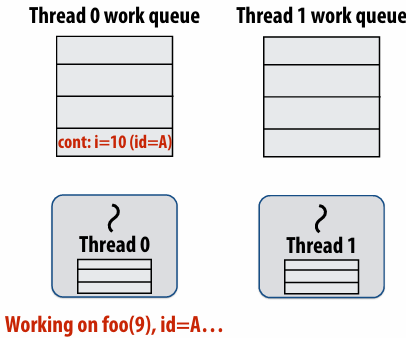
Note: descriptor(描述符) for block A created
The descriptor tracks the number of outstanding(未完成的) spawns for the block, and the number of those spawns that have completed
The 1 spawn tracked by the descriptor corresponds to foo(0) being run by thread 0. (Since the continuation is now owned by thread 1 after the steal.)
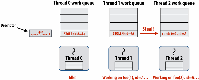
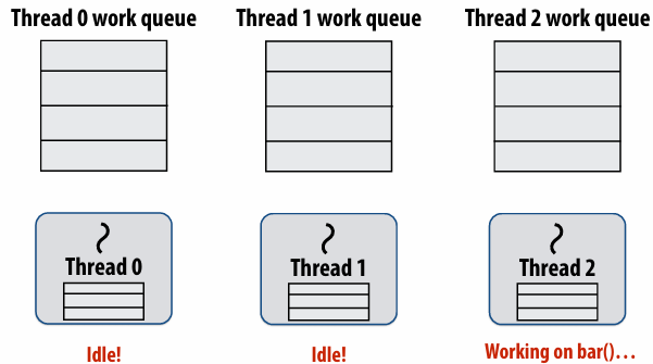
Thread 2 now resumes continuation and executes bar()
Note block A descriptor is now free
Cilk uses greedy join scheduling
Greedy join scheduling policy
All threads always attempt to steal if there is nothing to do
Threads only go idle if there is no work to steal in the system
Worker thread that initiated spawn may not be thread that executes logic after cilk_sync
Remember:
Overhead of bookkeeping(簿记) steals and managing sync points only occurs when steals occur
If large pieces of work are stolen, this should occur infrequently
Most of the time, threads are pushing/popping local work from their local dequeue
Cilk summary
Fork-join parallelism: a natural way to express divide-and-conquer algorithms
Discussed Cilk Plus, but many other systems also have fork/join primitives (e.g., OpenMP)
Cilk Plus runtime implements spawn/sync abstraction with a locality-aware(局部性感知) work stealing scheduler
Always run spawned child (continuation stealing)
Greedy behavior at join (threads do not wait at join, immediately look for other work to steal)
Lecture 6: Performance Optimization Part II: Locality, Communication, and Contention
shared address space model
Non-uniform memory access (NUMA)
The latency of accessing a memory location may be different from different processing cores in the system
Bandwidth from any one location may also be different to different CPU cores(In practice, you’ll find NUMA behavior on a single-socket system as well (recall: different cache slices are a different distance from each core))
Communication abstraction
Threads read/write variables in shared address space
Threads manipulate synchronization primitives: locks, atomic ops, etc
Logical extension of uniprocessor programming(But NUMA implementations require reasoning about locality for performance optimization)
Requires hardware support to implement efficiently
Any processor can load and store from any address
Can be costly to scale(扩展) to large numbers of processors(one of the reasons why high-core count processors are expensive)
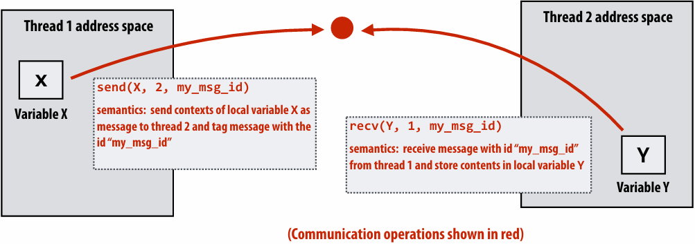
Message passing model
Message passing model (abstraction)
Threads operate within their own private address spaces
Threads communicate by sending/receiving messages
send: specifies(指定) recipient, buffer to be transmitted, and optional message identifier (“tag”)
receive: sender, specifies buffer to store data, and optional message identifier
Sending messages is the only way to exchange data between threads 1 and 2
Message passing (implementation)
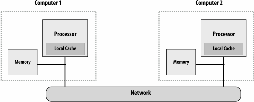
Hardware need not implement a single shared address space for all processors (it only needs to provide mechanisms to communicate messages between nodes)
Can connect commodity(通用) systems together to form a large parallel machine(message passing is a programming model for clusters and supercomputers)
Message passing expression of solver
Recall the grid solver application:
Update all red cells in parallel
When done updating red cells , update all black cells in parallel (respect dependency on red cells)
Repeat until convergence
Let’s think about expressing a parallel grid solver with communication via messages
One possible message passing machine configuration: a cluster of two machines
Message passing model: each thread operates in its own address space
In this figure: four threads
The grid data is partitioned into four allocations, each residing in one of the four unique thread address spaces
(four per-thread private arrays)
Data replication is now required to correctly execute the program
Grid data stored in four separate address spaces (four private arrays)
Message passing solver
Similar structure to shared address space solver, but now communication is explicit in message sends and receives
1 | int N; |
Notes on the message passing example
Computation
Array indexing is relative to local address space
Communication:
Performed by sending and receiving messages
Bulk(批量) transfer: communicate entire rows at a time
Synchronization:
Performed by sending and receiving messages
Consider how to implement mutual exclusion, barriers, flags using messages
Synchronous (blocking) send and receive
send(): call returns when sender receives acknowledgement that message data resides(存在) in address space of receiver
recv(): call returns when data from received message is copied into address space of receiver and acknowledgement sent back to sender
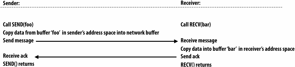
硬件确保 message 和 ack 传输成功
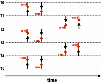
There is a big problem with our message passing solver if it uses synchronous send/recv
同时 send/receive 会导致 deadlock
Message passing solver (fixed to avoid deadlock)
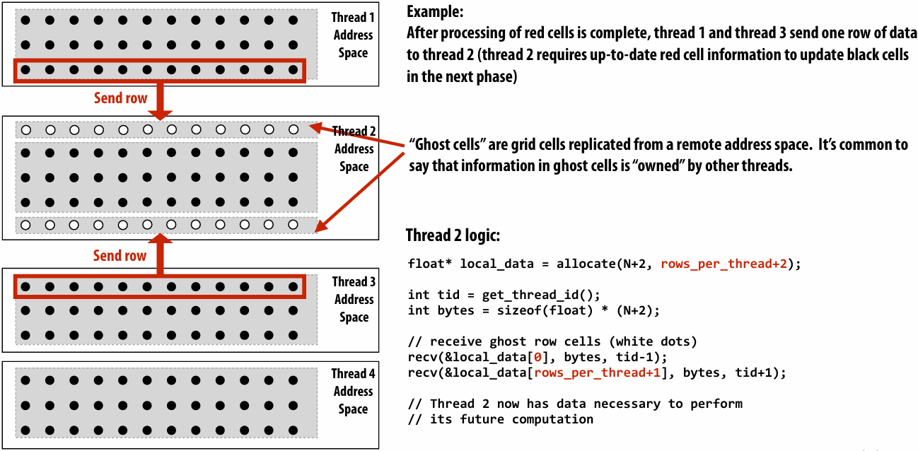
Send and receive ghost rows to “neighbor threads”
Even-numbered threads send, then receive
Odd-numbered thread recv, then send
1 | int N; |
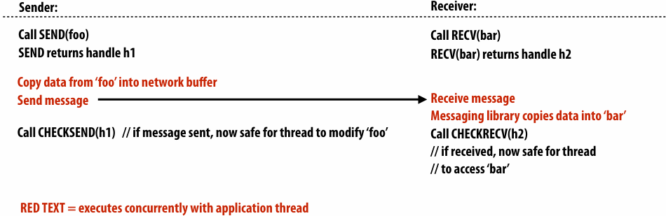
Non-blocking asynchronous send/recv
send(): call returns immediately
Buffer provided to send() cannot be modified by calling thread since message processing occurs concurrently with thread execution
Calling thread can perform other work while waiting for message to be sent
recv(): posts intent(意图) to receive in the future, returns immediately
Use checksend(), checkrecv() to determine actual status of send/receipt
Calling thread can perform other work while waiting for message to be received
When I talk about communication, I’m not just referring to messages between machines
More examples:
Communication between cores on a chip
Communication between a core and its cache
Communication between a core and memory
Think of a parallel system as an extended memory hierarchy(层次结构)
I want you to think of “communication” generally:
Communication between a processor and its cache
Communication between processor and memory (e.g., memory on same machine)
Communication between processor and a remote memory(e.g., memory on another node in the cluster, accessed by sending a network message)
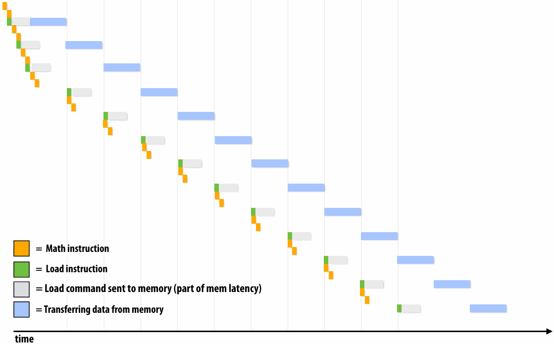
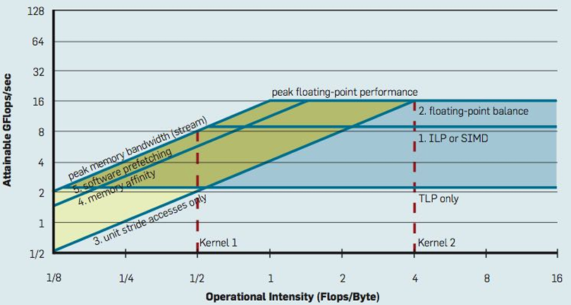
Discussion of bandwidth-limited execution (from lecture 3)
This was an example where the processor executed 2 instructions for each cache line load
How do you tell from the figure that the memory bus is fully utilized?
观察图中的蓝色长条(代表从内存传输数据的时间),在进入稳态(Steady State)后,发现一个蓝色长条的终点紧接着下一个蓝色长条的起点,没有间隙意味着内存总线在时间轴上是 100% 占满的。它始终在传输数据,没有任何空闲时间。即使核心(Core)在红色区域停顿(Stalled),内存总线依然在全力奔跑,说明总线被完全利用
How would you illustrate higher memory latency (keep in mind memory requests are pipelined and memory bus bandwidth is not changed)?
内存延迟 (Latency):从 CPU 发出内存请求到数据返回之间的等待时间
内存总线带宽 (Bandwidth):单位时间内内存系统能够传输的最大数据量
内存延迟体现在“发送加载命令(灰色)”到“数据开始传输(蓝色起始)”之间的间隔。如果延迟变高,这个间隔(灰色和蓝色之间的距离)会拉长。由于带宽没变,蓝色长条的宽度(长度)不会变。由于是流水线化的,只要请求够多,蓝色长条依然会保持“首尾相衔”。整排蓝色长条会相对于指令簇整体向右平移。在程序刚开始时,处理器等待第一份数据回来的时间(初始延迟)会变长,但一旦进入稳态,数据传输的频率(吞吐量)保持不变
How would the figure change if memory bus bandwidth was increased?
加带宽意味着在相同时间内可以传输更多数据,或者传输相同大小(一个缓存行)的数据所需的时间变短。每个蓝色长条会变窄(水平方向变短)。如果数学计算(黄色)的时间不变,蓝色长条变窄意味着数据回来的更快了,指令簇之间的空白区域(处理器停顿/Stalls)会缩小,整体执行速度加快
Would there still be processor stalls if the ratio of math instructions to load instructions was significantly increased? Why?
可能不会(停顿会消失),当每个加载指令对应的数学指令变多时,黄色长条的总长度(计算时间)会增加。如果计算时间长到足以覆盖掉数据传输的时间(蓝色长条的时间),那么当核心算完当前数据时,下一份数据已经传输完成了,此时程序从“访存受限(Memory-bound)”转变为“计算受限(Compute-bound)”。处理器始终在忙于计算,不再需要停下来等数据。即与计算强度(Arithmetic Intensity)有关
Arithmetic intensity
amount of computation (e.g., instructions) / amount of communication (e.g., bytes)
If numerator(分子) is the execution time of computation, ratio gives average bandwidth requirement of code(倒数)
1 / “Arithmetic intensity” = communication-to-computation ratio
Some people like to refer to communication to computation ratio
I find arithmetic intensity a more intuitive(直观) quantity, since higher is better
It also sounds cooler
High arithmetic intensity (low communication-to-computation ratio) is required to efficiently utilize modern parallel processors since the ratio of compute capability to available bandwidth is high (recall element-wise vector multiply example from lecture 3)
Two reasons for communication: inherent vs. artifactual communication
Inherent(固有) communication
Communication that must occur in a parallel algorithm
The communication is fundamental to the algorithm
In our messaging passing example at the start of class, sending ghost rows was inherent communication
Reducing inherent communication
Good assignment decisions can reduce inherent communication(increase arithmetic intensity)
1D blocked assignment: N x N grid 1D interleaved assignment: N x N grid

2D blocked assignment: N x N grid
N2 elements
P processors
elements computed(per processor): N2/P
elements communicated(per processor): 

arithmetic intensity:
Asymptotically(渐进地) better communication scaling than 1D blocked assignment
Communication costs increase sub-linearly(亚线性) with(随) P
Assignment captures 2D locality of algorithm
Artifactual(人工) communication
Inherent communication: information that fundamentally must be moved between processors to carry out the algorithm given the specified assignment (assumes unlimited capacity caches, minimum granularity transfers, etc.)
Artifactual communication: all other communication (artifactual communication results from practical details of system implementation)
Example: Artifactual communication arises from the behavior of caches
In this case: the communication is between memory and the processor
Data access in grid solver: row-major traversal
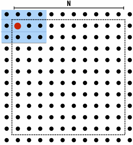
Assume row-major grid layout
Assume cache line is 4 grid elements
Cache capacity is 24 grid elements (6 lines)
Blue elements show data that is in cache after completing update to red element
Blue elements show data in cache at end of processing first row
Although elements (x,y)=(0,1), (1,1), (2,1), (0,2), and (2,2) have been accessed previously, they are no longer present in cache at start of processing the first output element in row 2
As a result, this program loads three cache lines for every four elements of output
Artifactual communication examples
System has minimum granularity of data transfer (system must communicate more data than what is needed by application)
Program loads one 4-byte float value but entire 64-byte cache line must be transferred from memory (16x more communication than necessary)
System operation might result in unnecessary communication:
Program stores 16 consecutive 4-byte float values, and as a result the entire 64-byte cache line is loaded from memory, entirely overwritten, then subsequently stored to memory (2x overhead… load was unnecessary since entire cache line was overwritten)
Finite replication capacity: the same data communicated to processor multiple times because cache is too small to retain it between accesses (capacity misses)
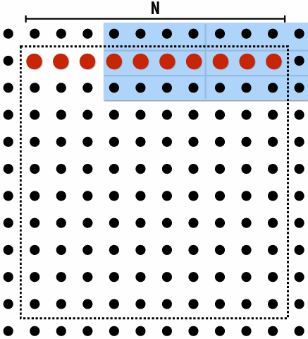
Techniques for reducing Artifactual communication
Improving temporal locality by changing grid traversal order
“Blocking”: reorder computation to reduce capacity misses
“Blocked” iteration order
(diagram shows state of cache after f inishing work from first row of first block)
Now load two cache lines for every six elements of output
Improving temporal(时间) locality by “fusing(融合)” loops
1 | // Two loads, one store per math op (arithmetic intensity = 1/3) |
1 | // Four loads, one store per 3 math ops (arithmetic intensity = 3/5) |
Code on top is more modular(模块化) (e.g, array-based math library like numPy in Python)
Code on bottom performs much better
Optimization: improve arithmetic intensity by sharing data
Exploit sharing: co-locate(共同定位) tasks that operate on the same data
Schedule threads working on the same data structure at the same time on the same processor
Reduces inherent communication
Contention
A resource can perform operations at a given throughput (number of transactions per unit time)
Memory, communication links, servers, CA’s at office hours, etc
Contention occurs when many requests to a resource are made within a small window of time(the resource is a “hot spot”)
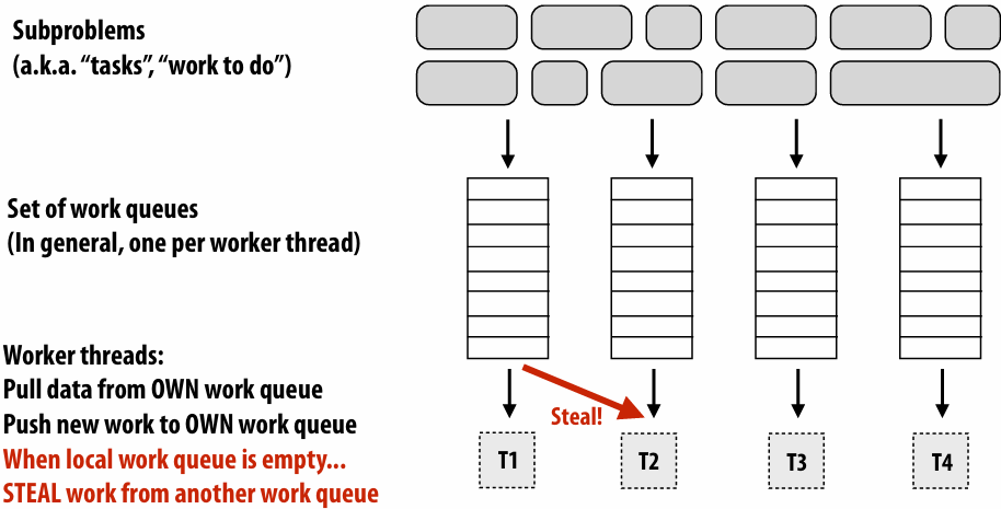
Example: distributed work queues reduce contention(contention in access to single shared work queue)
Worker threads:
Pull data from OWN work queue
Push new work to OWN work queue
(no contention when all processors have work to do)
When local work queue is empty…
STEAL work from random work queue
(synchronization okay at this point since the thread would have sat idle anyway)
Summary: reducing communication costs
Reduce overhead of communication to sender/receiver
Send fewer messages, make messages larger (amortize(分摊) overhead)
Coalesce(合并) many small messages into large ones
Reduce latency of communication
Application writer: restructure code to exploit locality
Hardware implementor: improve communication architecture
Reduce contention
Replicate contended resources (e.g., local copies, fine-grained(细粒度) locks)
Stagger(错开) access to contended resources
Increase communication/computation overlap(重叠)
Application writer: use asynchronous communication (e.g., async messages)
Requires additional concurrency in application (more concurrency than number of execution units)
Here are some tricks for understanding the performance of parallel software
Remember: Always, always, always try the simplest parallel solution first, then measure performance to see where you stand
A useful performance analysis strategy
Determine if your performance is limited by computation, memory bandwidth (or memory latency), or synchronization?
Try and establish “high watermarks”
What’s the best you can do in practice?
How close is your implementation to a best-case scenario?
Roofline model
In plot below, different points on the X axis correspond to different programs with different arithmetic intensities
The Y axis is the maximum obtainable instruction throughput for a program with a given arithmetic intensity
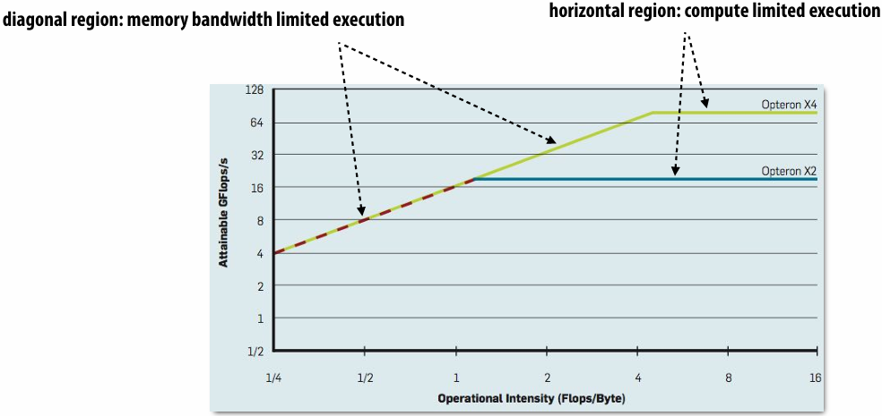
斜率是带宽(bandwidth)
Roofline model: optimization regions
Use various levels of optimization in benchmarks(基准)(e.g., best performance with and without using SIMD instructions)
Establishing high watermarks
Computation, memory access, and synchronization are almost never perfectly overlapped. As a result, overall performance will rarely be dictated(决定) entirely by compute or by bandwidth or by sync. Even so, the sensitivity of performance change to the above program modifications can be a good indication of dominant costs
Add “math” (non-memory instructions)
Does execution time increase linearly with operation count as math is added?(If so, this is evidence that code is instruction-rate limited)
Remove almost all math, but load same data
How much does execution time decrease? If not much, you might suspect memory bottleneck
Change all array accesses to A[0]
How much faster does your code get? (This establishes an upper bound on benefit of improving locality of data access)
Remove all atomic operations or locks
How much faster does your code get? (provided(假设) it still does approximately the same amount of work)(This establishes an upper bound on benefit of reducing sync overhead.)
Use profilers/performance monitoring tools
Image is “CPU usage(使用率)” from activity monitor in OS X while browsing the web in Chrome (from a laptop with a quad-core Core i7 CPU)
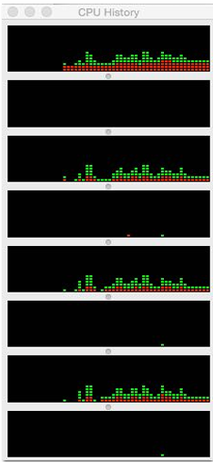
Graph plots(绘制) percentage of time OS has scheduled a process thread onto a processor execution context
Not very helpful for optimizing performance
All modern processors have low-level event “performance counters”
Registers that count important details such as: instructions completed, clock ticks, L2/L3 cache hits/misses, bytes read from memory controller, etc
Example: Intel’s Performance Counter Monitor Tool provides a C++ API for accessing these registers
1 | PCM *m = PCM::getInstance(); |
Also see Intel VTune, PAPI, oprofile, etc
Understanding problem size issues can very helpful when assessing program performance
Understanding scaling
There can be complex interactions(交互) between the size of the problem to solve and the size of the parallel computer
Can impact load balance, overhead, arithmetic intensity, locality of data access
Effects can be dramatic and application dependent
Evaluating a machine with a fixed problem size can be problematic
Too small a problem:
Parallelism overheads dominate(掩盖) parallelism benefits (may even result in slow downs)
Problem size may be appropriate for small machines, but inappropriate for large ones (does not reflect realistic usage of large machine!)
Too large a problem: (problem size chosen to be appropriate for large machine)
Key working set may not “fit” in small machine (causing thrashing to disk, or key working set exceeds cache capacity, or can’t run at all)
When problem working set “fits” in a large machine but not small one, super-linear speedups can occur
Can be desirable to scale problem size as machine sizes grow
(buy a bigger machine to compute more, rather than just compute the same problem faster)
Summary of tips
Measure, measure, measure…
Establish high watermarks for your program
Are you compute, synchronization, or bandwidth bound?
Be aware of scaling issues
Is the problem “well sized” for the machine?
Assignment 2: Scheduling Task Graphs on a Multi-Core CPU
具体内容和实现
[WorldClass/Stanford CS149 Parallel Computing/asst2 at master · tiny-star3/WorldClass](https://github.com/tiny-star3/WorldClass/tree/master/Stanford CS149 Parallel Computing/asst2)
Lecture 7: GPU Architecture & CUDA Programming
GPU compute mode
Review: how to run code on a CPU
Lets say a user wants to run a program on a multi-core CPU…
OS loads program text into memory
OS selects CPU execution context
OS interrupts processor, prepares execution context (sets contents of registers, program counter, etc. to prepare execution context)
Go!
Processor begins executing instructions from within the environment maintained in the execution context
How to run code on a GPU (prior to 2007)
Let’s say a user wants to draw a picture using a GPU…
Application (via graphics driver) provides GPU shader program binaries
Application sets graphics pipeline(管道) parameters (e.g., output image size)
Application provides GPU a buffer of vertices
Application sends GPU a “draw” command: drawPrimitives(vertex_buffer)
This was the only interface to GPU hardware
GPU hardware could only execute graphics pipeline computations
NVIDIA Tesla architecture (2007)
First alternative, non-graphics-specific (“compute mode”) interface to GPU hardware
Let’s say a user wants to run a non-graphics program on the GPU’s programmable cores…
Application can allocate buffers in GPU memory and copy data to/from buffers
Application (via graphics driver) provides GPU a single kernel program binary
Application tells GPU to run the kernel in an SPMD fashion (“run N instances of this kernel”) launch(myKernel, N)
Interestingly, this is a far simpler operation than the graphics operation drawPrimitives()
CUDA programming language
Introduced in 2007 with NVIDIA Tesla architecture
“C-like” language to express programs that run on GPUs using the compute-mode hardware interface
Relatively low-level: CUDA’s abstractions closely match the capabilities/performance characteristics of modern GPUs (design goal: maintain low abstraction distance)
CUDA programming abstractions
Describe CUDA abstractions using CUDA terminology
Specifically, be careful with the use of the term “CUDA thread”. A CUDA thread presents a similar abstraction as a pthread in that both correspond to logical threads of control, but the implementation of a CUDA thread is very different
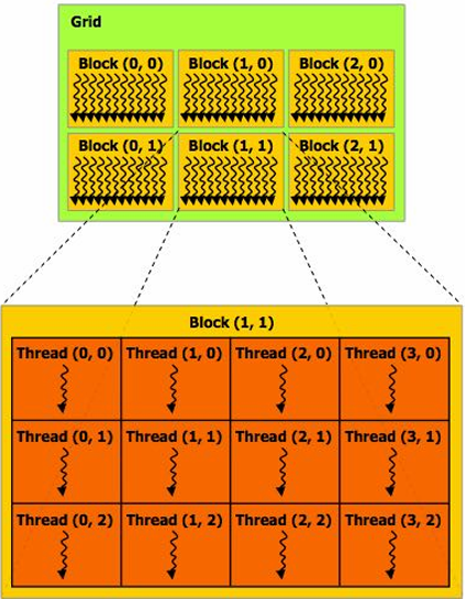
CUDA programs consist of a hierarchy of concurrent threads
Thread IDs can be up to 3-dimensional (2D example below)
Multi-dimensional thread ids are convenient for problems that are naturally N-D
Basic CUDA syntax
1 | // Regular application thread running on CPU (the “host”) |
1 | // SPMD execution of device kernel function: |
Clear separation of host and device code
Separation of execution into host and device code is performed statically by the programmer
Number of SPMD “CUDA threads” is explicit in the program
Number of kernel invocations(调用) is not determined by size of data collection(Block内都会调用)
(a kernel launch is not specified by map(kernel, collection) as was the case with graphics shader programming)
1 | // Regular application thread running on CPU (the “host”) |
1 | // CUDA kernel definition |
CUDA execution model
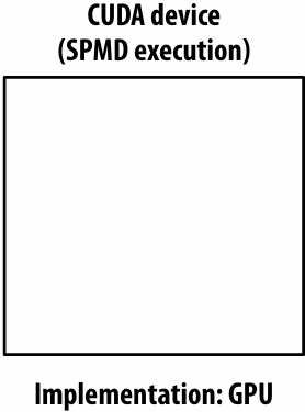
CUDA memory model
Distinct(独立的) host and device address spaces
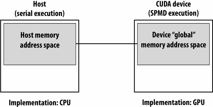
memcpy primitive
Move data between address spaces
1 | float* A = new float[N]; // allocate buffer in host mem |
CUDA device memory model
Three distinct types of address spaces visible to kernels
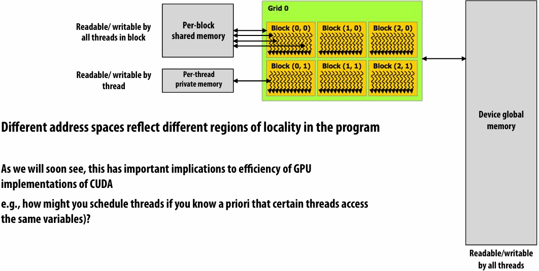
priori(先验)
CUDA example: 1D convolution(卷积)
output[i] = (input[i] + input[i+1] + input[i+2]) / 3.f;
1D convolution in CUDA (version 1)
One thread per output element
1 | // CUDA Kernel |
1 | // Host code |
1D convolution in CUDA (version 2)
One thread per output element: stage input data in per-block shared memory
1 | // CUDA Kernel |
1 | // Host code |
CUDA synchronization constructs
__syncthreads()
Barrier: wait for all threads in the block to arrive at this point
Atomic operations
e.g., float atomicAdd(float* addr, float amount)
CUDA provides atomic operations on both global memory addresses and per-block shared memory addresses
Host/device synchronization
Implicit barrier across all threads at return of kernel
Summary: CUDA abstractions
Execution: thread hierarchy
Bulk launch of many threads (this is imprecise… I’ll clarify later)
Two-level hierarchy: threads are grouped into thread blocks
Distributed address space
Built-in memcpy primitives to copy between host and device address spaces
Three different types of device address spaces
Per thread, per block (“shared”), or per program (“global”)
Barrier synchronization primitive for threads in thread block
Atomic primitives for additional synchronization (shared and global variables)
SPMD vs. SIMD
SPMD is a programming model question independent of the implementation
So like ISPC is an SPMD programming model, CUDA is a SPMD programming model
What that means is I write one program, like this program right here, and the system will run it many times with different thread IDs
Now how we execute all those threads or all those instances efficiently is up to the implementation
And ISPC use SIMD the instructions to execute things very efficiently
CUDA implementation on modern GPUs
CUDA semantics
1 |
|
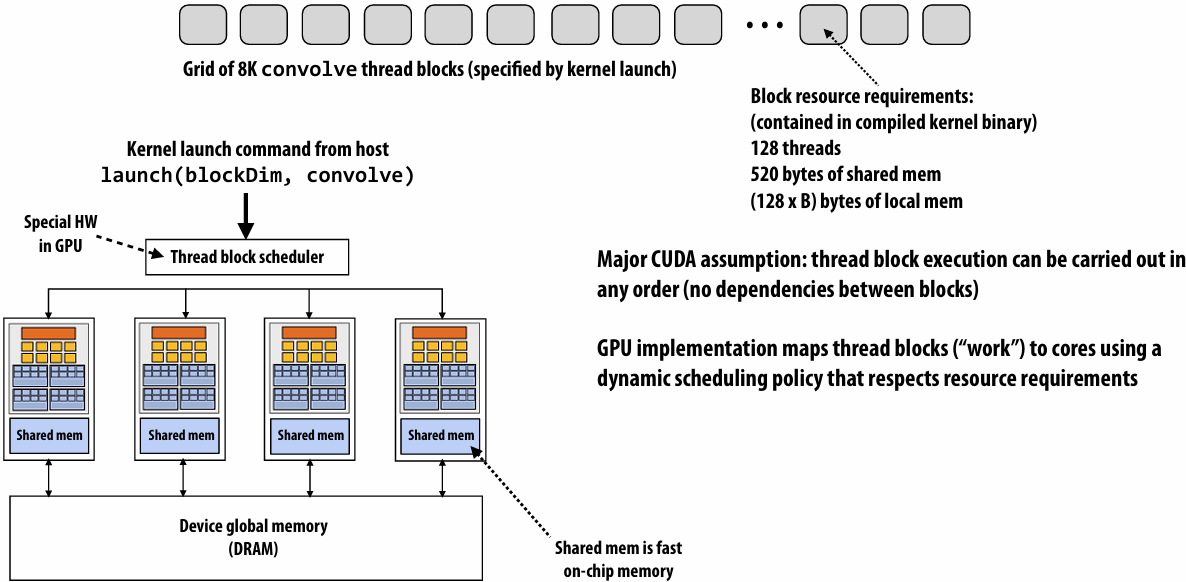
Assigning work
Desirable for CUDA program to run on all of these GPUs without modification
Note: there is no concept of num_cores in the CUDA programs I have shown you. (CUDA thread launch is similar in spirit to a forall loop in data parallel model examples)
CUDA compilation
A compiled CUDA device binary includes:
Program text (instructions)
Information about required resources:
128 threads per block
B bytes of local data per thread
128+2=130 floats (520 bytes) of shared space per thread block
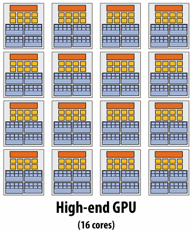
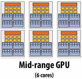
CUDA thread-block assignment
More detail on GPU architecture
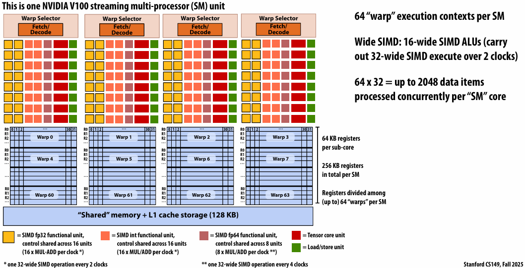
NVIDIA V100 SM “sub-core”
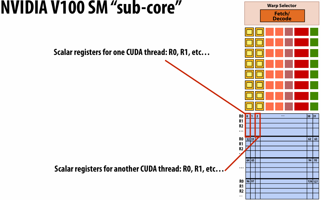
Threads in a warp are executed in a SIMD manner, **if they share the same instruction**
	NVIDIA calls this SIMT (single instruction multiple CUDA thread)
	If the 32 CUDA threads do not share the same instruction,  performance can suffer due to divergent execution
	This mapping is similar to how ISPC runs program instances in a gang(But GPU hardware is dynamically checking whether 32 independent CUDA threads share an instruction, and if this is true, it  executes all 32 threads in a SIMD manner.  The CUDA program is not compiled to SIMD instructions like ISPC gangs)(一个硬件实现,一个软件实现)
A warp is not part of CUDA, but is an important CUDA implementation  detail on modern NVIDIA GPUs
Instruction execution
Instruction stream for CUDA threads in a warp…
(note in this example all instructions are independent)
00 fp32 mul r0 r1 r2
01 int32 add r3 r4 r5
02 fp32 mul r6 r7 r8
…
Remember, entire warp of CUDA threads is running this instruction stream
So each instruction is run by all 32 CUDA threads in the warp
Since there are 16 ALUs, running the instruction for the entire warp takes two clocks
NVIDIA V100 GPU SM
This is one NVIDIA V100 streaming multi-processor (SM) unit
Running a thread block on a V100 SM
A convolve thread block is executed by 4 warps(4 warps x 32 threads/warp = 128 CUDA threads per block)
1 |
|
SM core operation each clock:
Each sub-core selects one runnable warp (from the 16 warps in its partition)
Each sub-core runs next instruction for the CUDA threads in the warp (this instruction may apply to all or a subset of the CUDA threads in a warp depending on divergence)
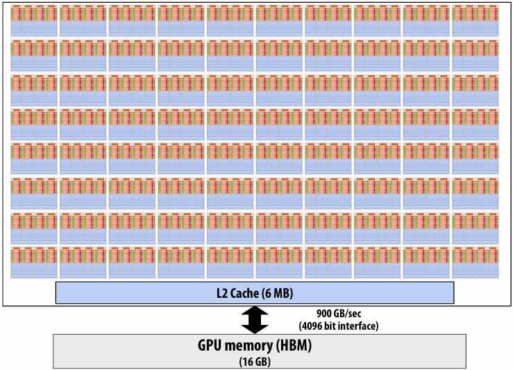
NVIDIA V100 GPU (80 SMs)
Summary: geometry of the V100 GPU
1.245 GHz clock
80 SM cores per chip
80 x 4 x 16 = 5,120 fp32 mul-add ALUs = 12.7 TFLOPs (mul-add counted as 2 flops)
Up to 80 x 64 = 5120 interleaved warps per chip (163,840 CUDA threads/chip)
Reminder: GPU “SIMT” (single instruction, multiple thread)
Running a CUDA program on a GPU
Running the convolve kernel
convolve kernel’s execution requirements:
Each thread block must execute 128 CUDA threads
Each thread block requires 130 x sizeof(float) = 520 bytes of shared memory
Let’s assume array size N is very large, so the host-side kernel launch generates thousands of thread blocks
#define THREADS_PER_BLK 128
convolve<<<N/THREADS_PER_BLK, THREADS_PER_BLK>>>(N, input_array, output_array);
Let’s run this program on the fictitious two-core GPU below
Running the CUDA kernel
Step 1: host sends CUDA device (GPU) a command (“execute this kernel”)
Step 2: scheduler maps block 0 to core 0 (reserves(预留) execution contexts for 128 threads and 520 bytes of shared storage)
Step 3: scheduler continues to map blocks to available execution contexts (interleaved mapping shown). Only two thread blocks fit on a core(third block won’t fit due to insufficient shared storage 3 x 520 bytes > 1.5 KB)
Step 4: thread block 0 completes on core 0
Step 5: block 4 is scheduled on core 0 (mapped to execution contexts 0-127)
Step 6: thread block 2 completes on core 0
Step 7: thread block 5 is scheduled on core 0 (mapped to execution contexts 128-255)
More advanced scheduling questions
(If you understand the following examples you really understand how CUDA programs run on a GPU, and also have a good handle on the work scheduling issues we’ve discussed in the course up to this point.)
Why must CUDA allocate execution contexts for all threads in a block?
Imagine a thread block with 256 CUDA threads
1 |
|
Assume a fictitious(虚拟的) SM core (shown above) with only 128 threads (four warps) worth of parallel execution in HW
Why not just run threads 0-127 to completion, then run threads 128-255 to completion in order to execute the entire thread block?
The idea is that the threads in a thread block are not just SPMD threads, but running concurrently at the same time, live at the same time on the same SM because you may do things like want them to cooperate with barriers or atomics and stuff like that
CUDA kernels may create dependencies between threads in a block
Simplest example is __syncthreads()
Threads in a block cannot be executed by the system in any order when dependencies exist
CUDA semantics: threads in a block ARE running concurrently. If a thread in a block is runnable it will eventually(最终) be run! (no deadlock)
Implementation of CUDA abstractions
Thread blocks can be scheduled in any order by the system
System assumes no dependencies between blocks
Logically concurrent
A lot like ISPC tasks, right?
CUDA threads in same block run concurrently (live at same time)
When block begins executing, all threads exist and have register state allocated(these semantics impose(强加) a scheduling constraint on the system)
A CUDA thread block is itself an SPMD program (like an ISPC gang of program instances)
Threads in thread block are concurrent, cooperating “workers”
CUDA implementation:
A NVIDIA GPU warp has performance characteristics akin(类似) to an ISPC gang of instances (but unlike an ISPC gang, the warp concept does not exist in the programming model(Exceptions(例外) to this statement include intra-warp(wrap内部) builtin(内置) operations like swizzle and vote))
All warps in a thread block are scheduled onto the same SM, allowing for high-BW(高带宽)/low latency communication through shared memory variables
When all threads in block complete, block resources (shared memory allocations, warp execution contexts) become available for next block
“persistent thread” CUDA programming style
1 |
|
Idea: write CUDA code that requires knowledge of the number of cores and blocks per core that are supported by underlying GPU implementation
Programmer launches exactly as many thread blocks as will fill the GPU
(Program makes assumptions about GPU implementation: that GPU will in fact run all blocks concurrently. Ugg!)
Now, work assignment to blocks is implemented entirely by the application(circumvents(规避) GPU’s thread block scheduler)
Now the programmer’s mental model is that all CUDA threads are concurrently running on the GPU at once
CUDA summary
Execution semantics
Partitioning of problem into thread blocks is in the spirit of the data-parallel model (intended to be machine independent: system schedules blocks onto any number of cores)
Threads in a thread block actually do run concurrently (they have to, since they cooperate)
Inside a single thread block: SPMD shared address space programming
There are subtle(微妙的), but notable(显著的) differences between these models of execution. Make sure you understand it. (And ask yourself what semantics are being used whenever you encounter a parallel programming system)
Memory semantics
Distributed address space: host/device memories
Thread local/block shared/global variables within device memory
Loads/stores move data between them (so it is correct to think about local/shared/global memory as being distinct(不同的) address spaces)
Key implementation details:
Threads in a thread block are scheduled onto same GPU “SM” to allow fast communication through shared memory
Threads in a thread block are are grouped into warps for SIMT execution on GPU hardware
Lecture 8: Data-Parallel Thinking
Think about describing algorithms in terms of(按照) operations on sequences of data
map sort filter groupBy(分组) fold / reduce(归约) join scan / segmented scan partition / flatten(展平)
Main idea: high-performance parallel implementations of these operations exist. So programs written in terms of these primitives can often run efficiently on a parallel machine(if you can avoid being bandwidth bound)
Motivation
Why must an application expose large amounts of parallelism?
Utilize large numbers of cores
High-core count machines
Many machines (e.g., cluster of machines in the cloud)
SIMD processing + multi-threaded cores require even more parallelism
GPU architectures require very large amounts of parallelism
Recall: geometry of the V100 GPU
1.245 GHz clock
80 SM cores per chip
80 x 4 x 16 = 5,120 fp32 mul-add ALUs = 12.7 TFLOPs(mul-add counted as 2 flops)
Up to 80 x 64 = 5120 interleaved warps per chip (163,840 CUDA threads/chip)
This chip can concurrently execute up to 163,860 CUDA threads! (programs that do not expose significant amounts of parallelism, and don’t have high arithmetic intensity, will not run efficiently on GPUs!)
Understanding dependencies is key
Key part of parallel programming is understanding when dependencies exist between operation
Lack of dependencies implies potential for parallel execution
Data-parallel model
Organize computation as operations on sequences of elements
e.g., perform same function on all elements of a sequence
A well-known modern example: NumPy: C = A + B
(A, B, and C are vectors of same length)
Key data type: sequences
Ordered collection of elements
In a C++ like language: Sequence<T\>
Scala lists: List[T]
Python Pandas Dataframes
PyTorch/JAX Tensors (N-D sequences)
In a functional language (like Haskell): seq T
Important: unlike arrays, programs only access elements of a sequence through specific operations, not direct element access
Map
Map
Higher order function(高阶函数) (function that takes a function as an argument)
Applies side-effect(副作用) free unary(一元) function f :: a -> b to all elements of input sequence, producing output sequence of the same length
In a functional language (e.g., Haskell)
map :: (a -> b) -> seq a -> seq b
In C++:
template<class InputIt, class OutputIt, class UnaryOperation\>
OutputIt transform(InputIt first1, InputIt last1, OutputIt d_first, UnaryOperation unary_op);
In JAX: vmap
1 | int f(int x) { return x + 10; } |
1 | a = [3, 8, 4, 6, 3, 9, 2, 8] |
Parallelizing map
Since f :: a -> b is a function (side-effect free), then applying f to all elements of the sequence can be performed in any order without changing the output of the program
Therefore, the implementation of map has flexibility to reorder/parallelize processing of elements of sequence however it sees fit(根据需要)
map f s =
partition sequence s into P smaller sequences
for each subsequence s_i (in parallel)
out_i = map f s_i
out = concatenate out_i’s
Fold
Fold (fold left)
Apply binary operation f to each element and an accumulated value
Seeded by initial value of type b
f :: (b,a) -> b
1 | // E.g. |
Parallel fold
Apply f to each element and an accumulated value
In addition to binary(二元) function f, also need an additional binary “combiner(组合器)” function(No need for comb if f::(b,b)->b is an associative(结合律) binary operator) (不需要满足交换律)
Seeded by initial value of type b (must be identity for f and comb)
f :: (b,a) -> b
comb :: (b,b) -> b
fold_par :: b -> ((b,a) -> b) -> ((b,b)->b) ->seq a -> b
Scan
Scan
“scan inclusive”
f :: (a,a) -> a (associative binary op)
scan :: a -> ((a,a) -> a) -> seq a -> seq a
1 | // implement scan sequentially |
And so what scan computes is the repeated application of that operator up to and including the current element
Fold produces a single value, scan gives you all the partials
Alternative form(另一种形式): “scan exclusive”: out[i] is the scan result for all elements up to, but excluding, in[i]
Parallel Scan
Data-parallel scan
let A = [a0, a1, a2, a3, …, an-1]
let ⊕ be an associative binary operator with identity element(单位元素) I
scan_inclusive(⊕, A) = [a0, a0⊕a1, a0⊕a1⊕a2, …
scan_exclusive(⊕, A) = [I, a0, a0⊕a1, …
If operator is +, then scan_inclusive(+,A) is called “a prefix sum”
prefix_sum(A) = [a0, a0+a1, a0+a1+a2, …
Data-parallel inclusive scan(Subtract original vector to get exclusive scan result: not shown)
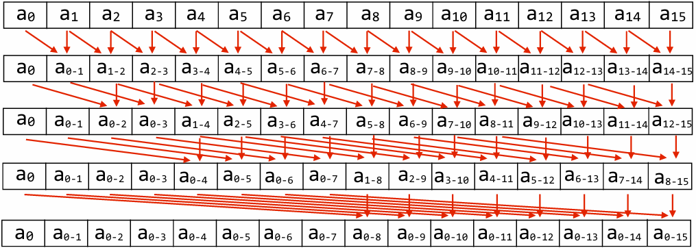
Work(Total operations performed): O(N lg N)
Span(Longest chain of sequential steps): O(lg N)
Inefficient compared to sequential algorithm!(工作量)
Work-efficient parallel exclusive scan (O(N) work)
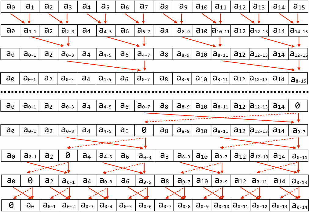
Work efficient exclusive scan algorithm(with ⊕ = “+”)
Up-sweep:
for d=0 to (log2n - 1) do
forall k=0 to n-1 by 2d+1 do
a[k + 2d+1 - 1] = a[k + 2d - 1] + a[k + 2d+1 - 1]
Down-sweep:
x[n-1] = 0
for d=(log2n - 1) down to 0 do
forall k=0 to n-1 by 2d+1 do
tmp = a[k + 2d - 1]
a[k + 2d - 1] = a[k + 2d+1 - 1]
a[k + 2d+1 - 1] = tmp + a[k + 2d+1 - 1]
Work: O(N) (but what is the constant?) 5
Span: O(lg N) (but what is the constant?) 2
Scan: two processor (shared memory) implementation
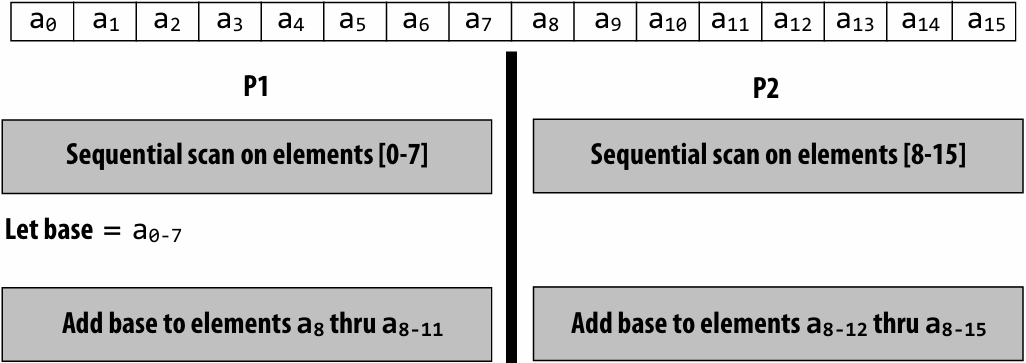
Work: O(N) (but constant is now only 1.5)
Data-access:
Very high spatial(空间) locality (contiguous memory access)
P1’s access to a8 through a8-11 may be more costly on large core count system with non-uniform(不均匀的) memory access costs, but on small-scale multi-core system the access cost is likely the same as from P2
Exclusive scan: SIMD implementation (in CUDA)
Example: perform exclusive scan on 32-element array: SPMD program, assume 32-wide SIMD execution
When scan_warp is run by a group of 32 CUDA threads, each thread returns the exclusive scan result for element idx(also: upon completionptr[]stores inclusive scan result)
1 | // 32-wide GPU execution (SPMD program) |
Work: N lg(N)
Work-efficient formulation of scan is not beneficial in this context because it results in low SIMD utilization
Work efficient algorithm would require more than 2x the number of instructions as the implementation above!
The fact that I did better would mean that I would have all this underutilization of my SIMD lanes, and so I do less work, but I spread it out over multiple highly incoherent instructions, so it’s a loss
Building scan on larger array
Example: 128-element scan using four-warp thread block
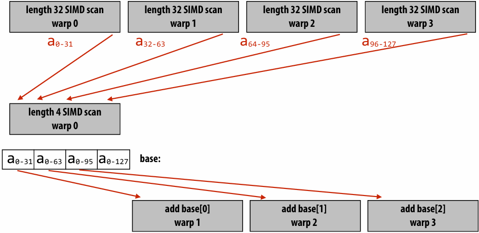
Multi-threaded, SIMD CUDA implementation
Example: cooperating threads in a CUDA thread block perform scan
We provide similar code in assignment 3
Code assumes length of array given by ptr is same as number of threads per block
1 | // idx: CUDA thread index of caller |
Building a larger scan
Example: one million element scan (1024 elements per block)
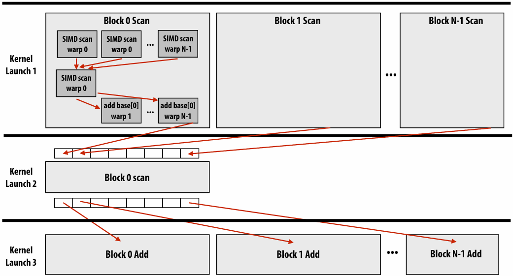
Exceeding 1 million elements requires partitioning phase two into multiple blocks
Scan implementation
Parallelism
Scan algorithm features O(N) parallel work
But efficient implementations only leverage(利用) as much parallelism as required to make good utilization of the machine
Goal is to reduce work and reduce communication/synchronization
Locality
Multi-level implementation to match memory hierarchy
(CUDA example: per-block implementation carried out in local memory)
Heterogeneity(异构性) in algorithm: different strategy for performing scan at different levels of the machine
CUDA example: different algorithm for intra-warp scan than inter-thread scan
Low-core count CPU example: based largely on sequential scan
Parallel Segmented Scan
Segmented scan
Common problem: operating on a sequence of sequences
Examples:
For each vertex v in a graph:
For each edge e connected to v
For each particle p in a simulation
For each particle within distance D of p
For each document d in a collection
For each word in d
There are two levels of parallelism in the problem that a programmer might want to exploit
But it is irregular: the size of edge lists, particle neighbor lists, words per document, etc, may be very different from vertex to vertex (or particle to particle)
Generalization(推广) of scan
Simultaneously(同时) perform scans on contiguous partitions of input sequence
let A = [ [1, 2], [6], [1, 2, 3, 4] ]
let ⊕ = +
segmented_scan_exclusive(⊕, A) = [[0,1], [0], [0,1,3,6]]
Assume a simple “start-flag” representation of nested(嵌套) sequences:
Consider nested sequence A = [[1,2,3],[4,5,6,7,8]]
flag: 1 0 0 1 0 0 0 0
data: 1 2 3 4 5 6 7 8
Work-efficient segmented scan(with ⊕ = “+”)
Up-sweep:
for d=0 to (log2n - 1) do:
forall k=0 to n-1 by 2d+1 do:
if flag[k + 2d+1 - 1] == 0:
data[k + 2d+1 - 1] = data[k + 2d - 1] + data[k + 2d+1 - 1]
flag[k + 2d+1 - 1] = flag[k + 2d - 1] || flag[k + 2d+1 - 1]
Down-sweep:
data[n-1] = 0
for d=(log2n - 1) down to 0 do:
forall k=0 to n-1 by 2d+1 do:
tmp = data[k + 2d - 1]
data[k + 2d - 1] = data[k + 2d+1 - 1]
if flag_original[k + 2d] == 1: # must maintain copy of original flags
data[k + 2d+1 - 1] = 0 # start of segment
else if flag[k + 2d - 1] == 1:
data[k + 2d+1 - 1] = tmp
else:
data[k + 2d+1 - 1] = tmp + data[k + 2d+1 - 1]
flag[k + 2d - 1] = 0
Segmented scan (exclusive)
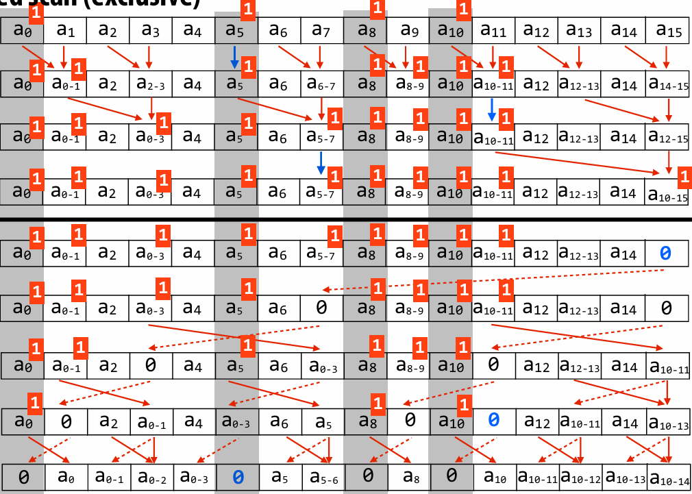
Scan/segmented scan summary
Scan
Theory: parallelism in problem is linear in number of elements
Practice: exploit locality, use only as much parallelism as necessary to fill the machine’s execution resources
Great example of applying different strategies at different levels of the machine
Segmented scan
Express computation and operate on irregular data structures (e.g., list of lists) in a regular, data parallel way
Gather/scatter: key data-parallel operations
gather(index, input, output)
output[i] = input[index[i]]
scatter(index, input, output)
output[index[i]] = input[i]
“Gather data from data_seq according to indices in index_seq”
output_seq = gather(index_seq, data_seq)
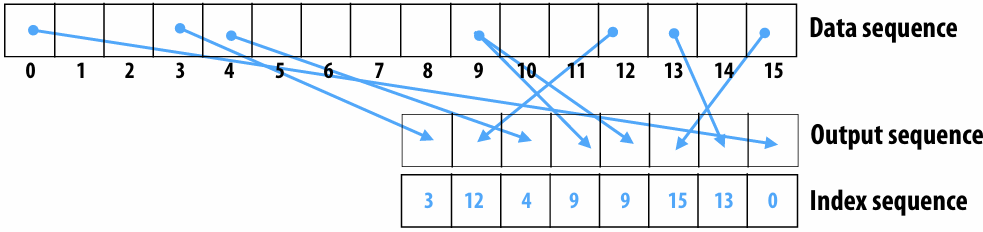
“Scatter data from data_seq according to indices in index_seq”
output_seq = scatter(index_seq, data_seq)
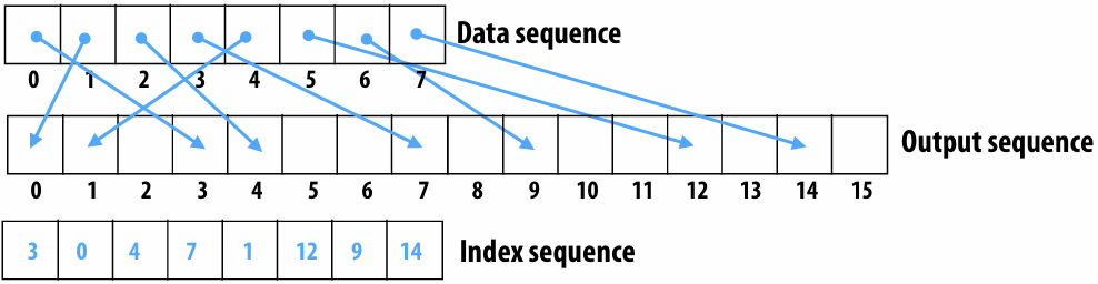
Gather machine instruction
“Gather from buffer mem_base into R1 according to indices specified by R0.”
gather(R1, R0, mem_base);
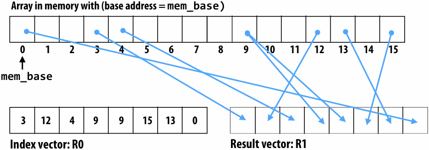
Gather supported with AVX2 in 2013
But AVX2 does not support SIMD scatter (must implement as scalar loop)
Scatter instruction exists in AVX512
Hardware supported gather/scatter exists on GPUs(still an expensive operation compared to load/store of contiguous vector)
Segmented scene + gather: sparse matrix multiplication example
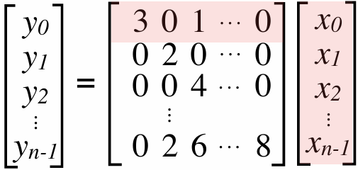
Most values in matrix are zero
Note: easy parallelization by parallelizing the different per-row dot products
But different amounts of work per row (complicates wide SIMD execution)
Example sparse storage format: compressed sparse row
values = [ [3,1], [2], [4], ..., [2,6,8] ]
cols = [ [0,2], [1], [2], ...., ]
row_starts = [0, 2, 3, 4, ... ]
Sparse matrix multiplication with scan
x = [x0,x1,x2,x3]
values = [ [3,1], [2], [4], [2,6,8] ]
cols = [ [0,2], [1], [2], [1,2,3] ]
row_starts = [0, 2, 3, 4]
1.Gather from x based on cols: gathered[i] = x[cols[I]]
gathered = [x0, x2, x1, x2, x1, x2, x3]
2.Map (multiplication) over all non-zero values: products[i] = values[i] * gathered[I]
products = [3x0, x2, 2x1, 4x2, 2x1, 6x2, 8x3]
3.Create flags vector from row_starts: flags = [1,0,1,1,1,0,0]
4.Perform inclusive segmented-scan on (products, flags) using addition operator
[3x0, 3x0+x2, 2x1, 4x2, 2x1, 2x1+6x2, 2x1+6x2+8x3]
5.Take last element in each segment:
y = [3x0+x2, 2x1, 4x2 , 2x1+6x2+8x3]
Turning a scatter into sort/gather
Special case: assume elements of index are unique and all elements referenced in index (scatter is a permutation)
scatter(index, input, output) {
output = sort input sequence by values in index sequence
}
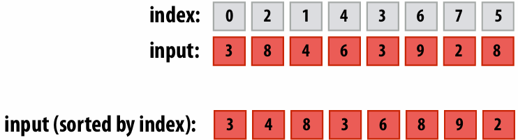
Implementing “scatterOp” with atomic sort/map/segmented-scan
Now, assume elements in index are not unique, so synchronization is required for atomicity!
for all elements in sequence
output[index[i]] = atomicOp(output[index[i]], input[i])
Example: atomicAdd(output[index[i], input[I]])
e.g,: index = [1, 1, 0, 2, 0, 0]
Step 1: Sort input sequence according to values in index sequence:
Sorted index: [0, 0, 0, 1, 1, 2]
Input sorted by index: [input[2], input[4], input[5], input[0], input[1], input[3]]
Step 2: Compute starts of each range of values with the same index number
starts: [1, 0, 0, 1, 0, 1]
Step 3: Segmented scan (using ‘op’) on each range
[op(op(input[2], input[4]), input[5]), op(input[0], input[1]), input[3])
More sequence operations
Group by key
Seq (key, T) —> Seq (key, Seq T)
Creates a sequence of sequences containing elements with the same key
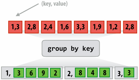
Filter
Remove elements from sequence that do not match predicate
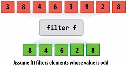
Sort
Example
Example: create grid of particles data structure on large parallel machine (e.g., a GPU)
Problem: place 1M point particles in a 16-cell uniform grid based on 2D position
Parallel data structure manipulation problem: build a 2D array of lists
Recall: Up to 2048 CUDA threads per SM core on a V100 GPU (80 SM cores)
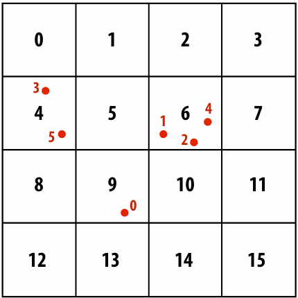
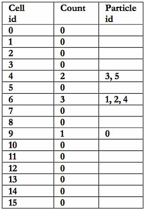
Common use of this structure: N-body problems
A common operation is to compute interactions(相互作用) with neighboring particles
Example: given a particle, find all particles within radius R
Organize particles by placing them in grid with cells of size R
Only need to inspect particles in surrounding grid cells
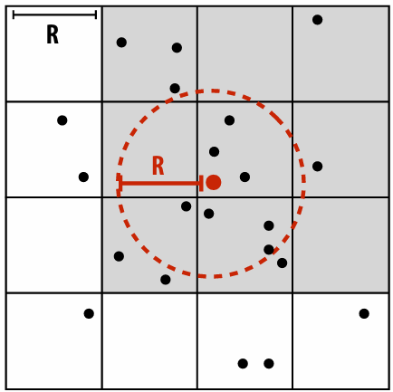
Solution 1: parallelize over particles
One answer: assign one particle to each CUDA thread. Each thread computes cell containing particle, then atomically updates per cell list
Problem: massive contention: thousands of threads contending for access to single shared data structure
1 | list cell_list[16]; // 2D array of lists |
Solution 2: use finer-granularity locks
Alleviate(缓解) contention for single global lock by using per-cell locks
Assuming uniform(均匀) distribution of particles in 2D space… ~16x less contention than previous solution
1 | list cell_list[16]; // 2D array of lists |
Solution 3: parallelize over cells
Decompose work by cells: for each cell, independently compute what particles are within it (eliminates contention because no synchronization is required)
Insufficient parallelism: only 16 parallel tasks, but need thousands of independent tasks to efficiently utilize GPU)
Work inefficient: performs 16 times more particle-in-cell computations than sequential algorithm
1 | list cell_lists[16]; // 2D array of lists |
Solution 4: compute partial results + merge
Yet another answer: generate N “partial” grids in parallel, then combine
Example: create N thread blocks (at least as many thread blocks as SM cores)
All threads in thread block update same grid
Enables faster synchronization: contention reduced by factor of N and cost of synchronization is lower because it is performed on block-local variables (in CUDA shared memory)
Requires extra work: merging the N grids at the end of the computation
Requires extra memory footprint(占用): stores N grids of lists, rather than 1
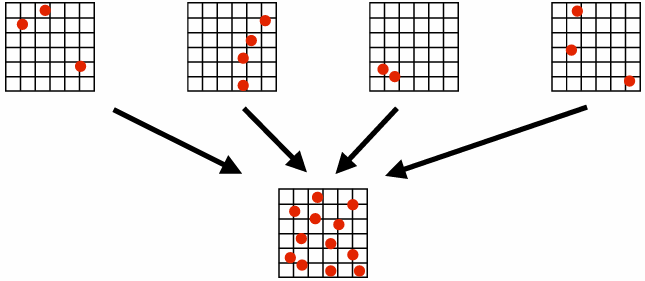
Solution 5: data-parallel approach
Step 1: map
compute cell containing each particle (parallel over input particles)
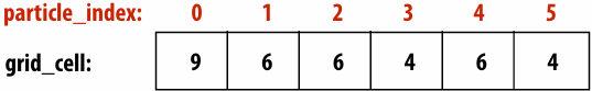
Step 2: sort results by cell (notice that the particle index array is also permuted(排列) based on sort)
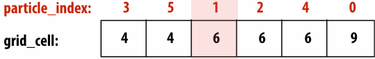
Step 3: find start/end of each cell (parallel over particle_index elements)
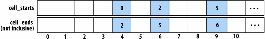
1 | // This code is run for each element of the particle_index array |
This solution maintains a large amount of parallelism and removes the need for fine-grained synchronization… at the cost of a sort and extra passes over the data (extra BW)!
Another example: parallel histogram
Consider computing a histogram for a sequence of values
1 | int f(float value); // maps array values to histogram bin id’s |
Challenge: create a massively parallel implementation of histogram given only map() and sort() on sequences
Data-parallel histogram construction
Assume variable thread_index is the “thread index” associated with the invocation of the kernel function
1 | void compute_bin(float* input, int* bin_ids) { |
Summary
Data parallel thinking:
Implementing algorithms in terms of simple (often widely parallelizable, efficiently implemented) operations on large data collections
Turn irregular parallelism into regular parallelism
Turn fine-grained synchronization into coarse synchronization
But most solutions require multiple passes over data — bandwidth hungry!
Data parallel primitives are basis for many parallel/distributed systems today
CUDA’s Thrust Library
Pandas Dataframe operations
JAX
Apache Spark / Hadoop
Lecture 9: Efficiently Evaluating DNNs
Review
When communication and computation are overlapped (hiding memory latency), the capabilities of the machine (ops throughput and communication bandwidth) AND the arithmetic intensity of the program determine if the program’s overall instruction throughput is limited by available bandwidth (“bandwidth bound”) or by the machine’s instruction processing capability (“compute bound”)
Overlapping communication and computation costs footprint, since buffers for the data being processing AND the data being transferred need to be maintained on chip
Increasing arithmetic processing ability (“faster hardware”) makes a program more likely to be bandwidth bound
Increasing a program’s arithmetic intensity (“a program change”) makes a program more likely to be compute bound
Mini-intro(简要介绍): Convolutional Neural Networks
What is a deep neural network?
A basic unit:
Unit with n inputs described by n+1 parameters(weights + bias)
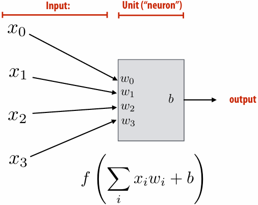
Example: rectified(修正) linear unit (ReLU) f(x)=max(0,x)
Basic computational interpretation:
It is just a circuit!
Machine learning interpretation:
Binary classifier: interpret output as the probability of one class
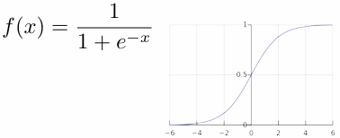
Deep neural network: topology(拓扑)
Fully connected layer as matrix-vector product
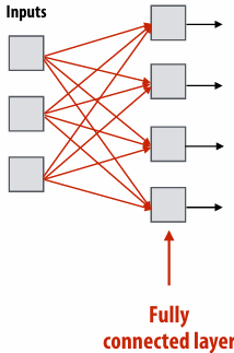
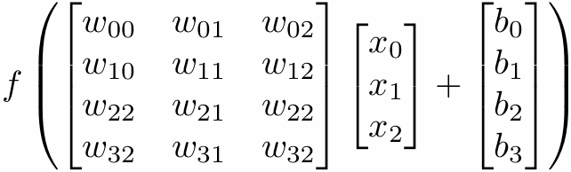
Assume f() is the element-wise max function (ReLU)
Image convolution (3x3 conv)
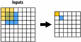
Convolutional layer: locally connected AND all units in layer share the same parameters (same weights + same bias)
1 | int WIDTH = 1024; |
Note: you can think of a filter as a “detector” of a pattern, and the magnitude(强度) of a pixel in the output image as the “response” of the filter to the region surrounding each pixel in the input image
Applying many filters to an image at once
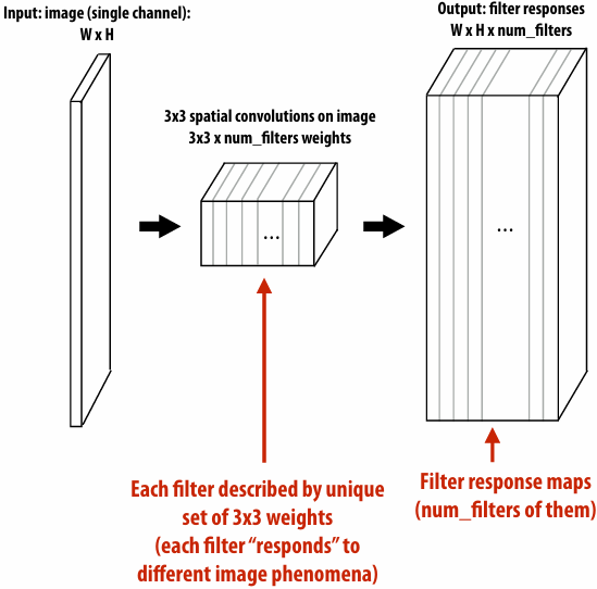
Adding additional layers
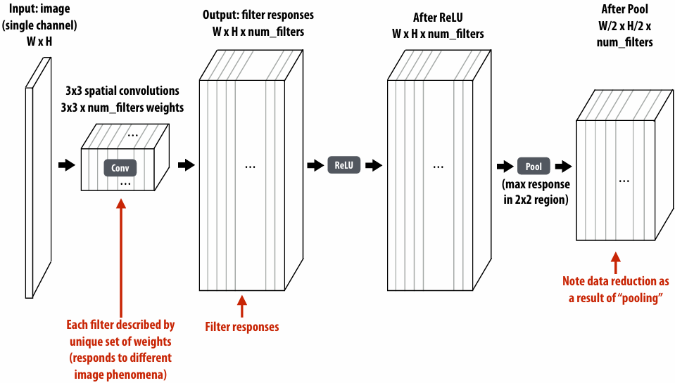
Efficiently implementing convolution layers
Direct implementation of conv layer (batched)
1 | float input[IMAGE_BATCH_SIZE][INPUT_HEIGHT][INPUT_WIDTH][INPUT_DEPTH]; // input activations(激活值) |
Seven loops with significant input data reuse: reuse of filter weights (during convolution), and reuse of input values (across different filters)
3x3 convolution as matrix-vector product (“explicit gemm”)
Construct matrix from elements of input image
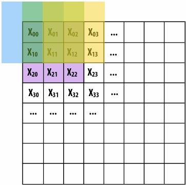
Note: 0-pad matrix
O(N) storage overhead for filter with N elements
Must construct input data matrix
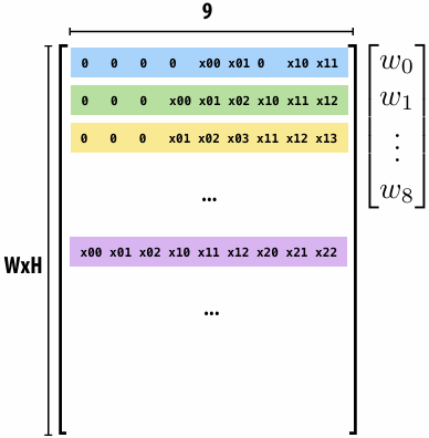
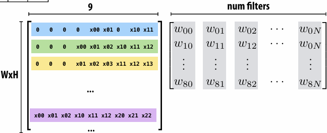
Multiple convolutions on multiple input channels
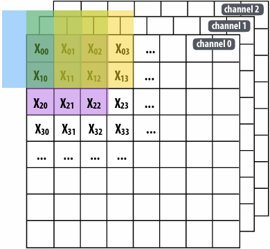
For each filter, sum responses over input channels
Equivalent to (3 x 3 x num_channels) convolution on (W x H x num_channels) input data
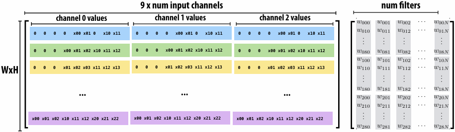
Conv layer to explicit GEMM mapping
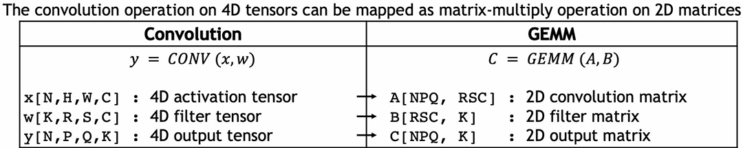
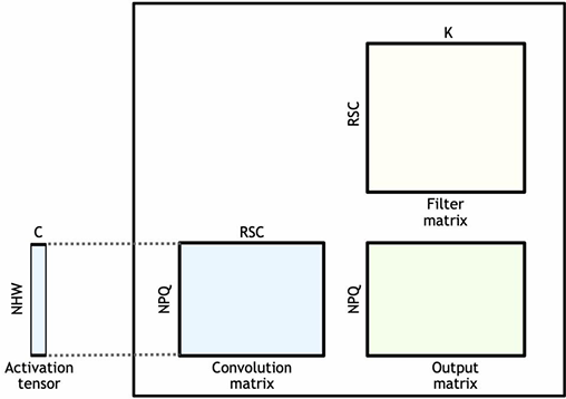
Symbol reference(符号参考):
Spatial support of filters: R x S
Input channels: C
Number of filters: K
Batch size: N
Matrix multiplication is at the heart of the “attention” blocks of a transformer architecture
Matrix multiplication is at the heart of the “attention” blocks of a transformer architecture
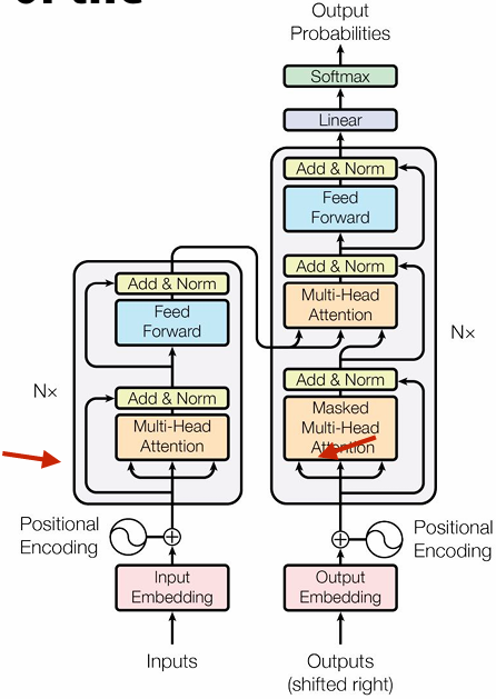
Sequence of tokens in, sequence of tokens out
The importance of dense matrix-matrix multiplication (GEMM) to modern AI
The kernel for…
Fully-connected layers
Convolutional layers
The attention block of a transformer
High performance implementations of GEMM exist
cuBLAS | NVIDIA Developer
Accelerate Fast Math with Intel® oneAPI Math Kernel Library
To use “off the shelf(现成的)” libraries, must materialize input matrices
For convolutional layer implications(影响), Increases DRAM traffic(流量) by a factor of R x S (To read input data from activation tensor and constitute “convolution matrix” )
Also requires large amount of additional storage
Dense matrix multiplication
1 | float A[M][K]; |
Low arithmetic intensity (does not exploit temporal locality in access to A and B)
Increasing arithmetic intensity by “blocking”
1 | float A[M][K]; |
Idea: compute partial result for block of C while required blocks of A and B remain in cache (Assumes BLOCKSIZE chosen to allow block of A, B, and C to remain resident)
Hierarchical blocked matrix mult
Exploit multiple levels of memory hierarchy (increase arithmetic intensity when considering multiple levels of memory hierarchy)
1 | float A[M][K]; |
Not shown: final level of “blocking” for register locality…
Vectorized, blocked dense matrix multiplication (1)
Consider SIMD parallelism within a block
1 | ... |
Vectorize i loop
Good: also improves spatial locality in access to B
Bad: working set increased by SIMD_WIDTH, still walking over B in large steps
Vectorized, blocked dense matrix multiplication (2)
1 | ... |
Assume i dimension is small
Previous vectorization scheme (1) would not work well
Pre-transpose(预转置) block of B (copy block of B to temp buffer in transposed form)
Vectorize innermost loop
Vectorized, blocked dense matrix multiplication (3)
1 | // assume blocks of A and C are pre-transposed as Atrans and Ctrans |
Different layers of a single DNN may benefit from unique scheduling strategies (different matrix dimensions)
Notice sizes of weights and activations in this network: (and consider SIMD widths of modern machines)
Ug for library implementers!
Matrix multiplication implementations
Optimization: do not materialize full matrix (“implicit gemm”)
This is a naive implementation that does not perform blocking, but indexes into input weight and activation tensors
Symbol reference:
Spatial support of filters: R x S
Input channels: C
Number of filters: K
Batch size: N
Better implementation: materialize only a sub-block of the convolution matrix at a time in GPU on-chip “shared memory”
Does not require additional off-chip storage and does not increase required DRAM traffic
Use well-tuned(良好调优) shared-memory based GEMM routines to perform sub-block GEMM (see CUTLASS)
Symbol reference:
Output size: PxQ
Spatial support of filters: R x S
Input channels: C
Number of filters (output channels): K
Batch size: N
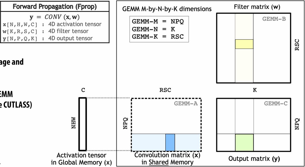
NVIDIA CUTLASS
Basic primitives/building block for implementing your custom high performance DNN layers. (e.g, unusual sizes that haven’t been heavily tuned by cuDNN)
NVIDIA/cutlass: CUDA Templates and Python DSLs for High-Performance Linear Algebra
Fast (in-shared memory) GEMM
Fast WARP level GEMMs
Iterators for fast block loading/tensor indexing
Tensor reductions
Etc
Triton
Welcome to Triton’s documentation! — Triton documentation
Language support for operations that load/store tensors
Load “blocks” of data into GPU shared memory
Perform data-parallel operations on those block
Thunderkittens
CUDA library of useful tile-based(基于图块) programming primitives
Intended to make advanced developers (CS149-level folks) more productive writing blocked code
Async load/store of tiles
Support for advanced memory layouts (blocked tiles, interleaved elements, etc.)
HazyResearch/ThunderKittens: Tile primitives for speedy kernels
Recall: NVIDIA V100 GPU (80 SMs)
Many processing units and many tensor cores
Need “a lot of parallel work” to fill the machine
Higher performance with “more work”
N=1, P=Q=64 case:
64 x 64 x 128 x 1 = 524K outputs = 2 MB of output data (float32)
N=32, P=Q=256 case:
256 x 256 x 128 x 32 = 256M outputs = 1 GB of output data (float32)
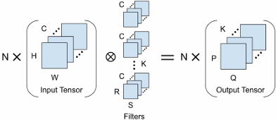
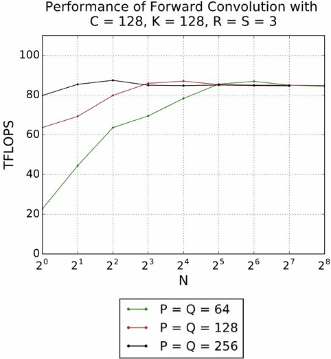
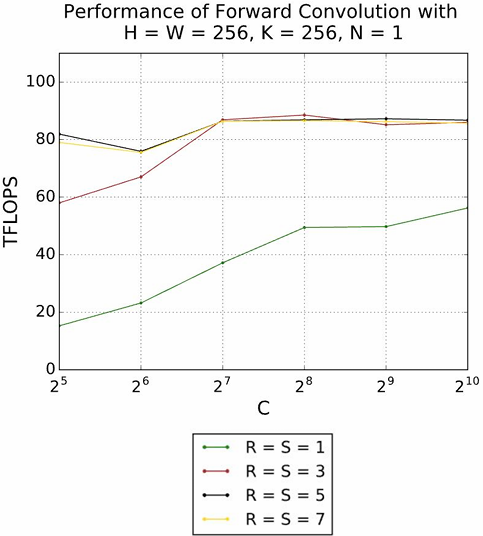
Direct implementation
Or you can just directly implement this loop nest directly yourself
1 | float input[IMAGE_BATCH_SIZE][INPUT_HEIGHT][INPUT_WIDTH][INPUT_DEPTH]; // input activations |
Low-level chip libraries offer high-performance implementations of key DNN layers
CUDA Deep Neural Network (cuDNN) | NVIDIA Developer
Intel® oneAPI Deep Neural Network Library (oneDNN)
Neuron Kernel Interface (NKI) Documentation — AWS Neuron Documentation
Libraries offering high-performance implementations of key DNN layers
torch.nn — PyTorch 2.9 documentation
Pytorch Convolution Layers -> NVIDIA cuDNN / Triton -> Graphics Card
Recall the loop fusion transformation: fuse multiple loops into one to increase a program’s arithmetic intensity
1 | // Program 1 |
1 | // Program 2 |
Memory traffic between operations
Consider this sequence:
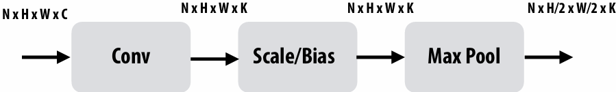
Imagine the bandwidth cost of dumping(存) 1 GB of conv outputs to memory, and then reading it back to just scale(缩放) all the values, and then rereading to perform the pool!
Better solution:
Per-element [scale+bias] operation can easily be performed per-element right after each element is computed by conv!
And max pool’s output can be computed once every 2x2 region of output is computed
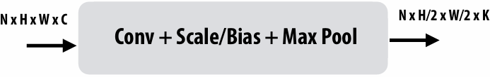
Fusing scale/bias with conv layer
1 | float input[IMAGE_BATCH_SIZE][INPUT_HEIGHT][INPUT_WIDTH][INPUT_DEPTH]; |
“fuse” a max pool operation following this layer (max of 2x2 blocks of output matrix)
1 | float input[IMAGE_BATCH_SIZE][INPUT_HEIGHT][INPUT_WIDTH][INPUT_DEPTH]; |
A good idea: fusion trick for computing “attention” in a modern transformer
Attention module in a modern transformer
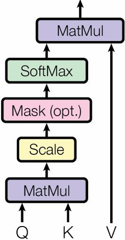
Let N be the length of the input sequence
Let d be the size of a feature embedding
Let Q be a N x d matrix
Let K be a N x d matrix
Let V be a N x d matrix
Let 
Let 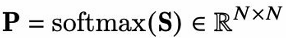 softmax(S) is computing softmax over the rows of S
Let 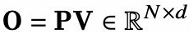
Notes:
N can be long for long sequences (e.g., thousands)
Naive implementation uses N2 space! Trouble!!!
Computing attention
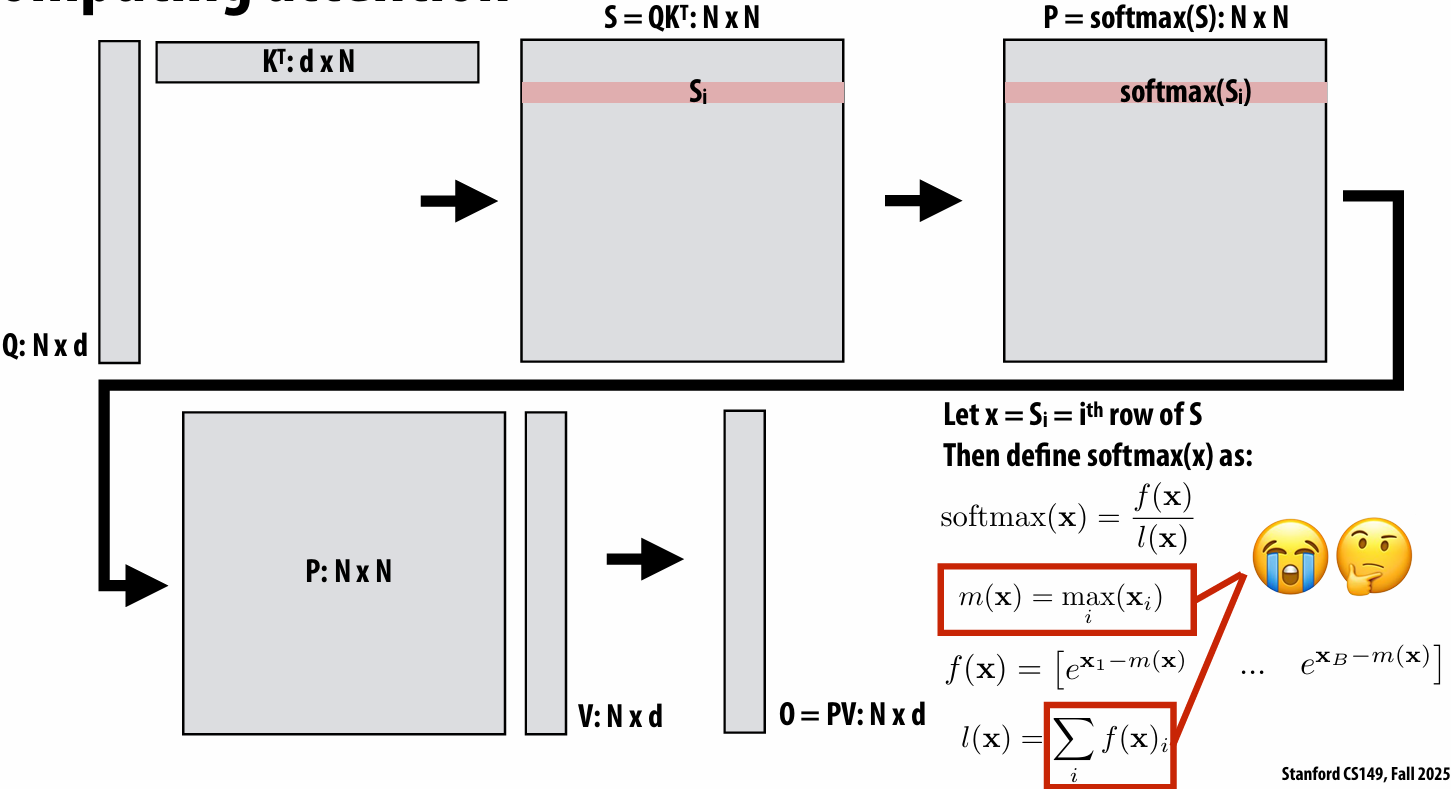
Let’s break vector x into chunks:
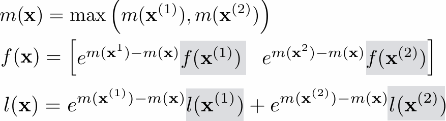
So softmax can be computed in chunks!
Fused attention
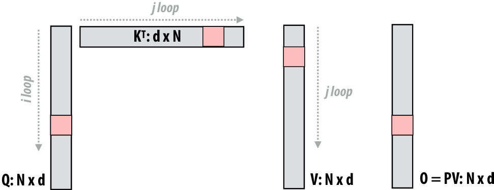
for each j:
for each i:
Load block Qi, KTj, Vj, Oi
Compute Sij = QiKTj
Compute Mij = m(Sij), Pij = f(Sij), and lij = l(Sij) (all functions operate row-wise on row-vectors)
Multiply PijVj and accumulate into Oi with appropriate scalings
Save memory footprint: Never materialize N2 matrix
Save memory bandwidth: (high arithmetic intensity)
Read 3 blocks (from Q, K, V)
Do two matrix multiplies + a few row summations
Accumulate into O block (which is resident in cache)
Note there is additional computation vs. the original version (must re-scale prior values of O each step of i-loop)
Fusion in modern DNN frameworks
Old style: library writers hardcoded a few “fused” ops
eg.
cudnnConvolutionBiasActivationForward
tensorflow::ops::FusedBatchNorm
tensorflow::ops::FusedResizeAndPadConv2D
More flexible fusion example: CUDNN “backend”
NVIDIA cuDNN Backend — NVIDIA cuDNN Backend
Compiler generates new implementations that “fuse” multiple operations into a single node that executes efficiently (without runtime overhead or communicating intermediate results through memory)
Many compiler-based efforts to automatically schedule key DNN operations
facebookresearch/TensorComprehensions: A domain specific language to express machine learning workloads.
JAX:高性能数组计算 — JAX 文档
apache/tvm: Open Machine Learning Compiler Framework
torch.compile 简介 — PyTorch 教程 2.9.0+cu128 文档 - PyTorch 文档
NervanaSystems/ngraph: nGraph has moved to OpenVINO
TensorRT SDK | NVIDIA Developer
triton-lang/triton: Development repository for the Triton language and compiler
Another trick: use of low precision values
Many efforts to use low precision values for DNN weights and intermediate activations
16 bit and 8-bit values are common
Now moving into 4 bit values
In the extreme case: 1-bit ;-)
[1603.05279] XNOR-Net: ImageNet Classification Using Binary Convolutional Neural Networks
[2509.25149] Pretraining Large Language Models with NVFP4
Optimization techniques
Better algorithms: manually designing better ML models
Common parameters: depth of network, width of filters, number of filters per layer, convolutional stride, etc
Common to perform automatic search for efficient topologies(拓扑)
Software optimization: Good scheduling of performance-critical operations
Loop blocking/tiling, fusion
Typically optimized manually by humans (but significant research efforts to automate scheduling)
Forms of approximation: compressing models
Lower bit precision
**Why might a GPU be a good platform for DNN evaluation? **
consider: arithmetic intensity, SIMD, data parallelism, memory bandwidth requirements
Deep neural networks on GPUs
Many high-performance DNN implementations target GPUs
High arithmetic intensity matrix-matrix computations benefit from flop-rich(浮点运算能力丰富) GPU architectures
Highly-optimized library of kernels exist for GPUs (cuDNN)
Why might a GPU be a sub-optimal platform for DNN evaluation?
(Hint: is a general purpose processor really needed?)
Next time: maximizing efficiency via specialized hardware acceleration for DNN inference/training
Google TPU3 GraphCore IPU Apple Neural Engine Intel Deep Learning Inference Accelerator Cerebras Wafer Scale Engine
SambaNova Cardinal SN10 Ampere GPU with Tensor Cores
【2023】Lecture 9: Spark (Distributed Computing on a Cluster)
Why Use A Cluster?
Want to process 100TB of log data (1 day @Facebook)
On 1 node: scanning @ 50MB/s = 23 days
On 1000 nodes: scanning @ 50MB/s = 33 min
get I/O bandwidth
But, very hard to utilize 1000 or 100,000 nodes!
Hard to program 16,000 cores
Something breaks every hour
Need efficient, reliable and usable framework
Warehouse-Scale Computers (WSC)
Standard architecture:
Cluster of commodity(商用) Linux nodes (multicore x86)
Private memory ⇒ separate address spaces & separate OS
Ethernet network ⇒ >10–40Gb today
Cheap?
Built from commodity processors, networks & storage
1000s of nodes for < $10M
WSC network is customized and expensive
Use a supercomputer networking ideas to provide high bandwidth across the datacenter
How to organize computations on this architecture?
Mask issues such as load balancing and failures
Warehouse-Scale Cluster Node (Server)
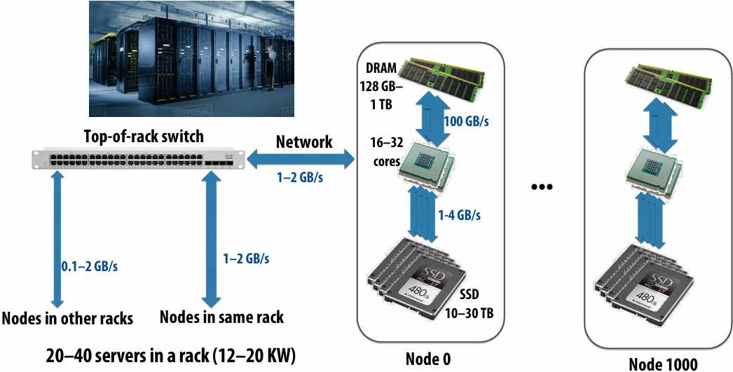
Consider bandwidths, what conclusions can you make?
In the early days, that was certainly not the case when you’re down at 0.1, but when you get up to the 2 gigabytes per second, now the picture is changing because now you can get potentially the same bandwidth to a remote nodes disk as to your local disk
Message passing model (abstraction)
Distributed memory communication without shared memory
Threads operate within their own private address spaces
Threads communicate by sending/receiving messages
send : specifies recipient, buffer to be transmitted, and optional message identifier (“tag”)
receive : sender, specifies buffer to store data, and optional message identifier
Sending messages is the only way to exchange data between threads 1 and 2
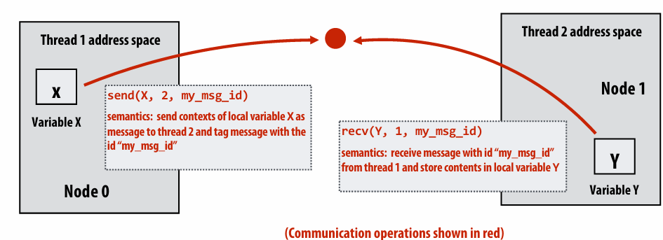
Do we need synchronization?
No because the act of sending a message is the synchronization
Storage Systems
First order problem: if nodes can fail, how can we store data persistently?
Answer: Distributed File System
Provides global file namespace
Google GFS, Hadoop HDFS
Typical usage pattern
Huge files (100s of GB to TB)
Data is rarely updated in place
Reads and appends are most common (e.g. log files)
Distributed File System (GFS)
Chunk servers
a.k.a. DataNodes in HDFS
File is split into contiguous chunks (usually 64–256 MB)
Each chunk replicated (usually 2x or 3x)
Try to keep replicas in different racks
Master node
a.k.a. NameNode in HDFS
Stores metadata; usually replicated
Client library for file access
Talks to master to find chunk (data) servers
Connects directly to chunk servers to access data
Hadoop Distributed File System (HDFS)
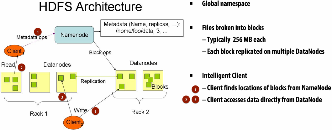
MapReduce Programming Model
Map
Higher order function(高阶函数) (function that takes a function as an argument)
Applies side-effect(副作用) free unary(一元) function f :: a -> b to all elements of input sequence, producing output sequence of the same length
In a functional language (e.g., Haskell)
map :: (a -> b) -> seq a -> seq b
In C++:
template<class InputIt, class OutputIt, class UnaryOperation\>
OutputIt transform(InputIt first1, InputIt last1, OutputIt d_first, UnaryOperation unary_op);
1 | int f(int x) { return x + 10; } |
1 | a = [3, 8, 4, 6, 3, 9, 2, 8] |
**Reduce **
Apply binary operation f to each element and an accumulated value
f :: (b,a) -> b
reduce :: ((b,a) -> b) -> seq a -> b
E.g., in Scala:
def reduce[A](f: (B, A) => B, l: List[A]): B
(The code above computes the count of page views by each type of mobile phone)
Assume cs149log.txt is a large file, stored in a distributed file system, like HDFS
Contents of cs149log.txt are distributed evenly in blocks across the cluster
1 | // called once per line in input file by runtime |
design an implementation of runMapReduceJob
MapReduce Dataflow for Word Count
Should be called MapGroupByKeyReduce
Step 1: Running the mapper function
Step 1: run mapper function on all lines of file
Question: How to assign work to nodes?
Idea 1: use work queue for list of input blocks to process
Dynamic assignment: free node takes next available block
Idea 2: data distribution based
assignment: Each node processes lines in blocks of input file that are stored locally
Steps 2 and 3: gathering data, running the reducer
Step 2: Prepare intermediate(中间的) data for reducer
Step 3: Run reducer function on all keys
Question: how to assign reducer tasks?
See what threads are spinning with no work to be done and are available, and assign it to them
Question: how to get all data for key onto the correct worker node?
use some hash function based on the key value and use that as the information given to the mapping task nodes, and that will indicate where those nodes should send the key value data to be reduced depending on the key
Additional implementation challenges at scale
Nodes may fail during program execution
Some nodes may run slower than others(due to different amounts of work, heterogeneity(异质性) in the cluster, etc..)
Job scheduler responsibilities
Exploit data locality: “move computation to the data”
Run mapper jobs on nodes that contain input blocks
Run reducer jobs on nodes that already have most of data for a certain key
Handling node failures
Scheduler detects job failures and reruns job on new machines
This is possible since inputs reside in persistent storage (distributed file system)
Scheduler duplicates jobs on multiple machines (reduce overall processing latency incurred by node failures)
Handling slow machines
Scheduler duplicates jobs on multiple machines
MapReduce Benefits
By providing a data-parallel model, MapReduce greatly simplified cluster programming:
Automatic division of job into tasks
Locality-aware scheduling
Load balancing
Recovery from failures & stragglers
runMapReduceJob problems
Permits only a very simple program structure
Programs must be structured as: map, followed by reduce by key
See DryadLINQ for generalization to DAGs
Iterative algorithms must load from disk each iteration
Example graph processing:
1 | void pagerank_mapper(graphnode n, map<string,string> results) { |
MapReduce Limitations
MapReduce greatly simplified “big data” analysis
But users quickly needed more:
More complex, multi-stage applications (e.g. iterative machine learning & graph processing)
More interactive ad-hoc(临时) queries
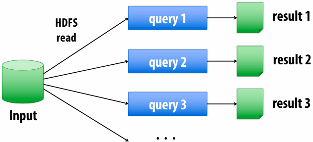
Application Trends
Despite huge amounts of data, many working sets in big data clusters fit in memory
Apache Spark in-memory, fault-tolerant distributed computing
Apache Spark™ - Unified Engine for large-scale data analytics
**Goals **
Programming model for cluster-scale computations where there is significant reuse of intermediate datasets
Iterative machine learning and graph algorithms
Interactive data mining: load large dataset into aggregate(聚合) memory of cluster and then perform multiple ad-hoc queries
Don’t want incur inefficiency of writing intermediates to persistent distributed file system (want to keep it in memory)
Challenge: efficiently implementing fault tolerance for large-scale distributed in-memory computations
Fault tolerance for in-memory calculations
Replicate all computations
Expensive solution: decreases peak throughput
Checkpoint and rollback
Periodically save state of program to persistent storage
Restart from last checkpoint on node failure
Maintain log of updates (commands and data)
High overhead for maintaining logs
Recall map-reduce solutions:
Checkpoints after each map/reduce step by writing results to file system
Scheduler’s list of outstanding(未完成的) (but not yet complete) jobs is a log
Functional structure of programs allows for restart at granularity of a single mapper or reducer invocation (don’t have to restart entire program)
Resilient Distributed Dataset (RDD)
Spark’s key programming abstraction :
Read-only ordered collection of records (immutable)
RDDs can only be created by deterministic(确定性) transformations on data in persistent storage or on existing RDDs
Actions on RDDs return data to application
1 | // create RDD from file system data |
Repeating the MapReduce Example
“Lineage”: Sequence of RDD operations needed to compute output
1 | // 1. create RDD from file system data |
Another Spark Program
1 | // create RDD from file system data |
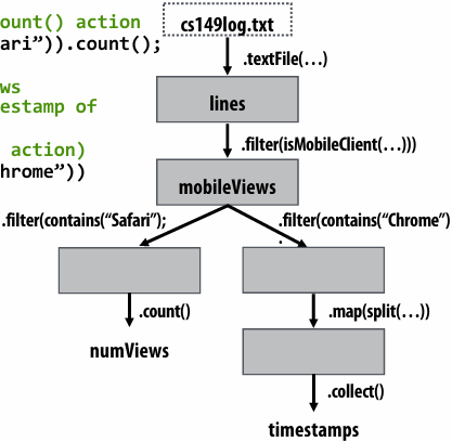
RDD transformations and actions
Transformations: (data parallel operators taking an input RDD to a new RDD)
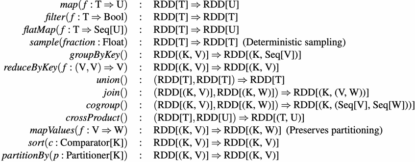
Actions: (provide data back to the “host” application)
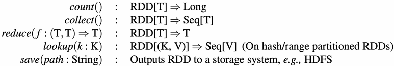
RDD partitioning and dependencies
val lines = spark.textFile(“hdfs://cs149log.txt”);
val lower = lines.map(_.toLower());
val mobileViews = lower.filter(x => isMobileClient(x));
val howMany = mobileViews.count();
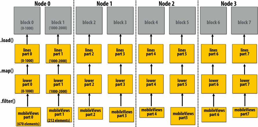
Black lines show dependencies between RDD partitions
**“loop fusion” & “tiling” **
globally restructuring the order of computation to improve producer-consumer locality
(improve arithmetic intensity of program)
Fusion with RDDs
Implementing sequence of RDD ops efficiently
The following code stores only a line of the log file in memory, and only reads input data from disk once (“streaming” solution)
1 | int count = 0; |
Narrow dependencies
“Narrow dependencies” = each partition of parent RDD referenced by at most one child RDD partition
Allows for fusing of operations (here: can apply map and then filter all at once on input element)
In this example: no communication between nodes of cluster (communication of one int at end to perform count() reduction)
Wide dependencies
groupByKey: RDD[(K,V)] → RDD[(K,Seq[V])]
“Make a new RDD where each element is a sequence containing all values from the parent RDD with the same key.”
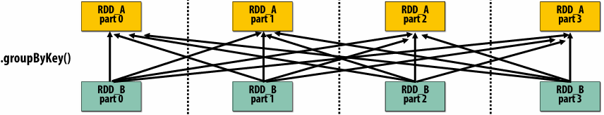
Wide dependencies = each partition of parent RDD referenced by multiple child RDD partitions Challenges:
Must compute all of RDD_A before computing RDD_B
Example: groupByKey() may induce all-to-all communication as shown above
May trigger significant recomputation of ancestor lineage upon node failure
Cost of operations depends on partitioning
join: RDD[(K,V)], RDD[(K,W)] → RDD[(K,(V,W))]
Assume data in RDD_A and RDD_B are partitioned by key: hash username to partition id
RDD_A and RDD_B have different hash partitions: join creates wide dependencies
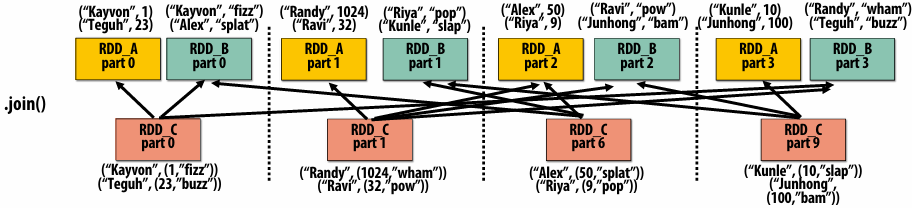
RDD_A and RDD_B have same hash partition: join only creates narrow dependencies
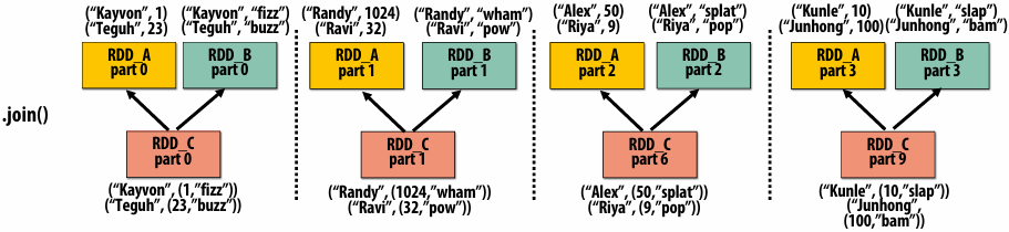
PartitionBy() transformation
Inform Spark on how to partition an RDD
e.g., HashPartitioner, RangePartitioner
1 | // create RDD from file system data |
.persist():
Inform Spark this RDD’s contents should be retained in memory
.persist(RELIABLE) = store contents in durable storage (like a checkpoint)
Implementing Resilience via Lineage
RDD transformations are bulk, deterministic, and functional
Implication: runtime can always reconstruct contents of RDD from its lineage(the sequence of transformations used to create it)
Lineage is a log of transformations
Efficient: since the log records bulk data-parallel operations, overhead of logging is low (compared to logging fine-grained operations, like in a database)
1 | // create RDD from file system data |
Upon Node Failure: Recompute Lost RDD Partitions from Lineage
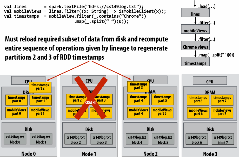
Note: (not shown): file system data is replicated so assume blocks 2 and 3 remain accessible to all nodes
Spark performance
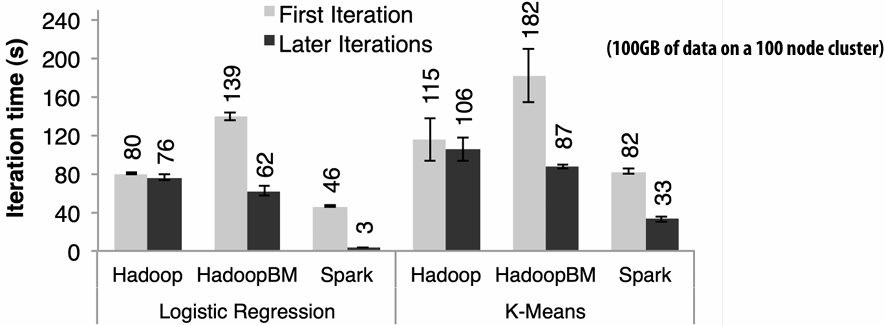
HadoopBM = Hadoop Binary In-Memory (convert text input to binary, store in in-memory version of HDFS)
the baseline parses text input in each iteration of an iterative algorithm
HadoopBM’s first iteration is slow because it runs an extra Hadoop job to copy binary form of input data to in memory HDFS
Accessing data from HDFS, even if in memory, has high overhead:
Multiple mem copies in file system + a checksum
Conversion from serialized form to Java object
Caution: “scale out” is not the entire story
People say scale out is when you are connecting nodes together by a network, and scale up is when you are connecting cores together in a shared memory system. So if you share a memory, it scale up. If you’re not sharing memory, it scale out
Distributed systems designed for cloud execution address many difficult challenges, and have been instrumental in the explosion of “big-data” computing and large-scale analytics
Scale-out parallelism to many machines
Resiliency in the face of failures
Complexity of managing clusters of machines
But scale out is not the whole story:
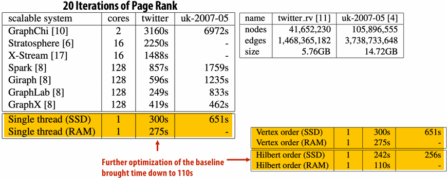
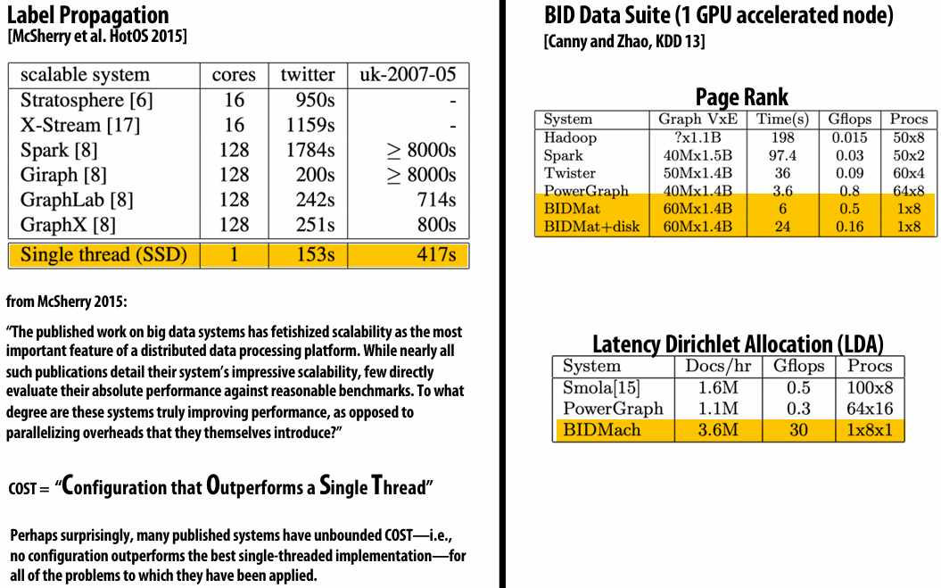
Performance improvements to Spark
With increasing DRAM sizes and faster persistent storage (SSD), there is interest in improving the CPU utilization of Spark applications
Goal: reduce “COST”
Efforts looking at adding efficient code generation to Spark ecosystem (e.g., generate SIMD kernels, target accelerators like GPUs, etc.) to close the gap on single node performance
RDD storage layouts must change to enable high-performance SIMD processing (e.g., struct of arrays instead of array of structs)
See Spark’s Project Tungsten, Weld [Palkar Cidr ’17], IBM’s SparkGPU
High-performance computing ideas are influencing design of future performance-oriented distributed systems
Conversely(相反): the scientific computing community has a lot to learn from the distributed computing community about elasticity(弹性) and utility(实用) computing
Spark summary
Introduces opaque(不透明的) sequence abstraction (RDD) to encapsulate(封装) intermediates of cluster computations (previously… frameworks like Hadoop/MapReduce stored intermediates in the file system)
Observation: “files are a poor abstraction for intermediate variables in large-scale data-parallel programs”
RDDs are read-only, and created by deterministic data-parallel operators
Lineage tracked and used for locality-aware scheduling and fault-tolerance (allows recomputation of partitions of RDD on failure, rather than restore from checkpoint (Note that .persist(RELIABLE) allows programmer to request checkpointing in long lineage situations) )
Bulk operations allow overhead of lineage tracking (logging) to be low
Simple, versatile(通用的) abstraction upon which many domain-specific distributed computing frameworks are being implemented
See Apache Spark project: spark.apache.org
Modern Spark ecosystem
Compelling(引入注目的) feature: enables integration(集成)/composition of multiple domain-specific frameworks (since all collections implemented under the hood with RDDs and scheduled using Spark scheduler)
Spark SQL
https://spark.apache.org/sql/
Interleave computation and database query
Can apply transformations to RDDs produced by SQL queries
Spark MLlib
https://spark.apache.org/mllib/
Machine learning library build on top of Spark abstractions
Spark GraphX
https://spark.apache.org/graphx/
GraphLab-like library built on top of Spark abstractions
Lecture 10: Hardware Specialization
Heterogeneous processing
Observation: most “real world” applications have complex workload characteristics
They have components that can be widely parallelized
And components that are difficult to parallelize
They have components that are amenable(易于相处的) to wide SIMD execution
And components that are not (divergent(发散的) control flow)
They have components with predictable data access
And components with unpredictable access, but those accesses might cache well
Idea: the most efficient processor is a heterogeneous mixture of resources (“use the most efficient tool for the job”)
Examples of heterogeneity
Example: Intel “Skylake” (2015)
(6th Generation Core i7 architecture)
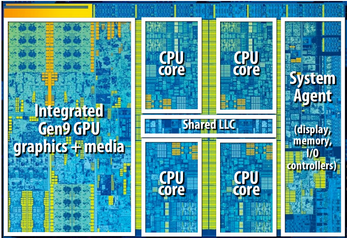
4 CPU cores + graphics cores + media accelerators
CPU cores and graphics cores share same memory system
Also share LLC (L3 cache)
Enables, low-latency, high-bandwidth communication between CPU and integrated(集成的) GPU
Graphics cores are cache coherent with CPU cores
More heterogeneity: add discrete(独立的) GPU
Keep discrete (power hungry) GPU unless needed for graphics-intensive applications
Use integrated, low power graphics for basic graphics/window manager/UI
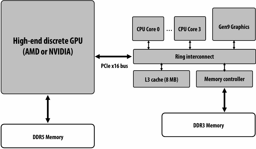
Mobile heterogeneous processors
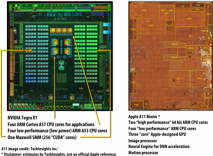
GPU-accelerated Supercomputing
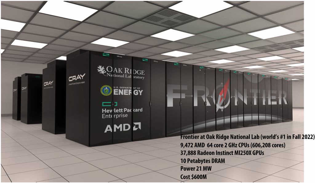
Energy-constrained computing
Energy (Power x Time)-constrained computing
Supercomputers are energy constrained
Due to shear(剪切) scale of machine (100,000s of CPUs and GPUs)
Overall cost to operate (power for machine and for cooling)
Datacenters are energy constrained
Reduce cost of cooling
Reduce physical space requirements
Mobile devices are energy constrained
Limited battery life
Heat dissipation(耗散)
AI is Constrained by Energy
AI demands are growing exponentially(呈指数级增长)
Data centers are heavily energy constrained

Performance and Power
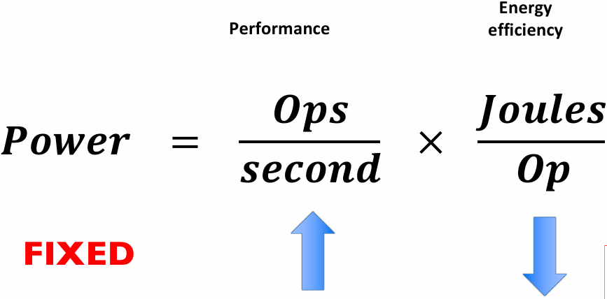
Better energy efficiency ⇒ Specialization (fixed function)
What is the magnitude of improvement from specialization?
Pursuing highly efficient processing… (specializing hardware beyond just parallel CPUs and GPUs)
Why is a “general-purpose processor” so inefficient?
Consider the complexity of executing an instruction on a modern processor…
Read instruction
Address translation, communicate with icache, access icache, etc.
Decode instruction
Translate op to uops, access uop cache, etc.
Check for dependencies/pipeline hazards(冲突)
Identify available execution resource
Use decoded operands to control register file SRAM (retrieve(检索) data)
Move data from register file to selected execution resource
Perform arithmetic operation
Move data from execution resource to register file
Use decoded operands to control write to register file SRAM
Review question:
How does SIMD execution reduce overhead of certain types of computations? What properties must these computations have?
amortize all of the parts that are not green over more green stuff. So you are executing across more data elements
Contrast that complexity to the circuit required to actually perform the operation
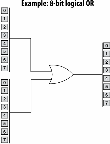
H.264 video encoding: fraction of energy consumed by functional units is small (even when using SIMD)
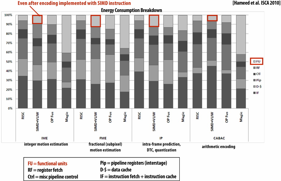
Fast Fourier(傅里叶) transform (FFT): throughput and energy benefits of specialization
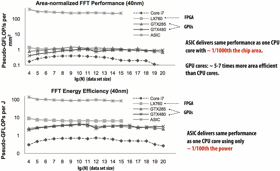
Mobile: benefits of increasing efficiency
Run faster for a fixed period of time
Run at higher clock, use more cores (reduce latency of critical task)
Do more at once
Run at a fixed level of performance for longer
e.g., video playback, health apps
Achieve “always-on” functionality that was previously impossible
iPhone:
Siri activated by button press or holding phone up to ear
Amazon Echo / Google Home
Always listening
Google Glass:
~40 min recording per charge (nowhere near “always on”)
Example: Intel “Skylake” (2015)
(6th Generation Core i7 architecture)
CPU cores and graphics cores share same memory system
Also share LLC (L3 cache)
Enables, low-latency, high-bandwidth communication between CPU and integrated(集成的) GPU
Graphics cores are cache coherent with CPU cores
GPU’s are themselves heterogeneous multi-core processors
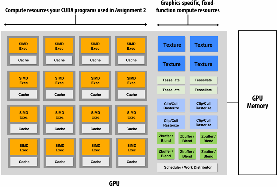
Example graphics tasks performed in fixed-function HW
Rasterization(光栅化): Determining what pixels a triangle overlaps

Texture mapping: Warping/filtering images to apply detail to surfaces

Geometric tessellation(镶嵌): computing fine-scale geometry from coarse geometry
Digital signal processors (DSPs)
Programmable processors, but simpler instruction stream control paths
Complex instructions (e.g., SIMD/VLIW): perform many operations per instruction (amortize cost of control)
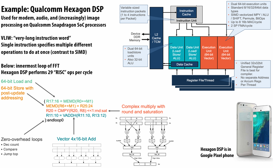
Anton supercomputer for molecular dynamics(分子动力学)
Anton 1 (2008) simulates time evolution of proteins(蛋白质)
ASIC for computing particle-particle interactions (512 of them in machine)
Throughput-oriented subsystem for efficient fast-fourier transforms
Custom, low-latency communication, network designed for communication patterns of N-body simulations
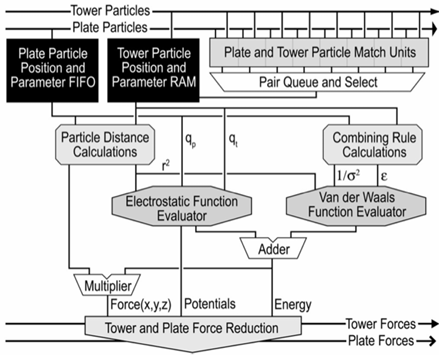
Anton 3 (2025) is approximately 20 times faster than a contemporary(当代的) GPU
Specialized processors for evaluating deep networks
Countless papers followed at top computer architecture research conferences on the topic of ASICs or accelerators for deep learning or evaluating deep networks…
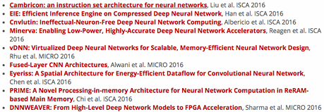
FPGAs (Field Programmable Gate Arrays)
Middle ground between an ASIC and a processor
FPGA chip provides array of logic blocks, connected by interconnect
Programmer-defined logic implemented directly by FGPA

Specifying combinational(组合) logic as a LUT(查找表)
Example: 6-input, 1 output LUT in Xilinx Virtex-7 FPGAs
Think of a LUT6 as a 64 elementtable
Example: 6-input AND
40-input AND constructed by chaining outputs of eight LUT6’s (delay = 3)
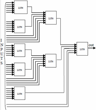
Modern FPGAs
A lot of area devoted to hard gates
Memory blocks (SRAM)
DSP blocks (multiplier)
CPUs (ARM, RISC-V)
Program with a hardware description language (e.g. Verilog, EE108)
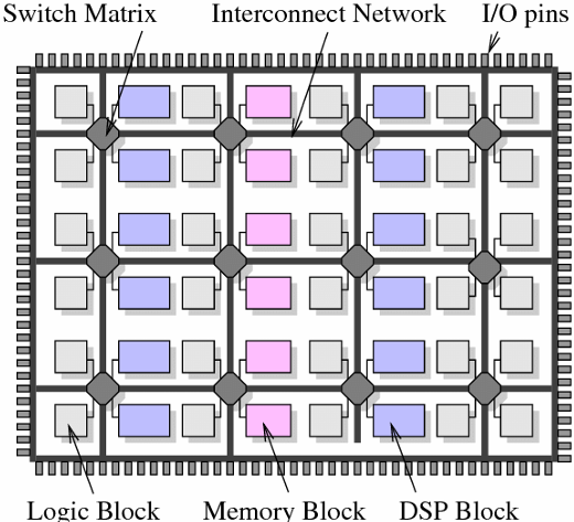
Amazon EC2 F1/F2
FPGA’s are now available on Amazon cloud services
https://aws.amazon.com/cn/ec2/
Efficiency benefits of compute specialization
Rules of thumb: compared to high-quality C code on CPU…
Throughput-maximized processor architectures: e.g., GPU cores
Approximately 10x improvement in perf / watt
Assuming code maps well to wide data-parallel execution and is compute bound
Fixed-function ASIC (“application-specific integrated circuit”)
Can approach 100-1000x or greater improvement in perf/watt
Assuming code is compute bound and is not floating-point math
Efficiency vs. Programability
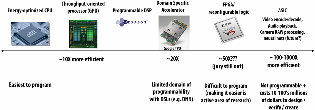
AI Progress Relies on Hardware Improvement
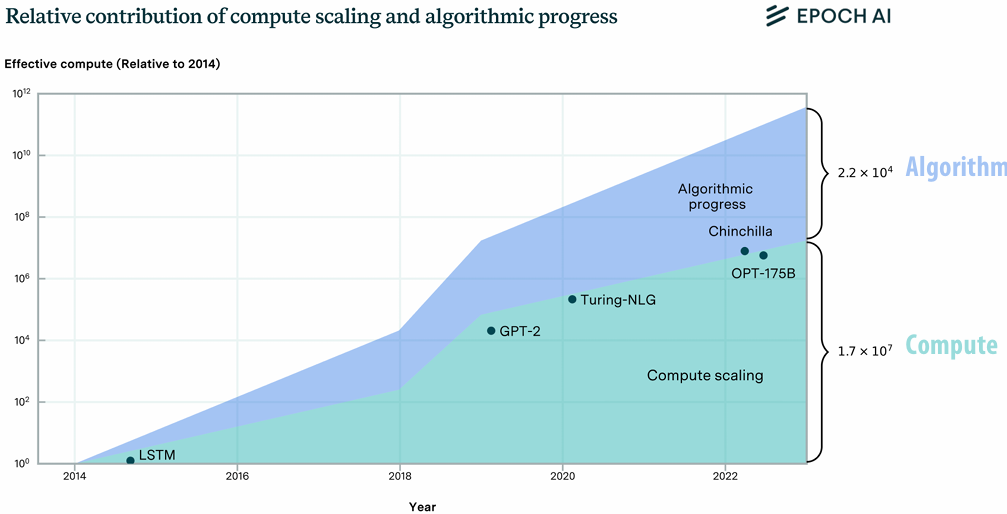
AI Models on GPUs
Many high-performance AI model implementations target GPUs
High arithmetic intensity computations (computational characteristics similar to dense matrix-matrix multiplication)
Benefit from flop-rich GPU architectures
Highly-optimized library of kernels exist for GPUs (cuDNN)
Why might a GPU be a sub-optimal platform for AI Model Acceleration?
(Hint: is a general purpose processor needed?)
Characteristics of An Ideal AI Model Accelerator
High peak TFLOPs and energy efficiency
High memory bandwidth
Simple to program for high-performance
Reaches performance bound on compute-bound models
Reaches performance bound on BW-bound models
Asynchronous (Nonblocking) Execution
Start later operations before earlier operations are complete
AI Models are Dataflow Graphs
Ideal AI Model Accelerator
Tiled(平铺式) AI accelerator programming model
CUTLASS
Triton
Thunderkittens
GEMM computation is cheap, but data movement is expensive
Silicon area
Watts
Nanoseconds
Ideal: Minimize cost of Data Movement
Ideal: Avoid Off-chip Data Access
| Feature | Why? |
|---|---|
| Tiled tensors (e.g. 16 x 16, 32 x 32) | Max TFLOPS on GEMM Low instr. overhead |
| Asynchronous compute | Overlap compute and memory access |
| Asynchronous memory access | Overlap compute and memory access |
| Asynchronous chip-to-chip communication | Overlap compute, memory and communication |
| Compute unit to compute unit comm. | Fusion and pipelining Streaming Dataflow |
Special instruction support
Recall: compute specialization = energy efficiency
Recall: data movement has high energy cost
Amortize overhead of instruction stream control using more complex instructions
Estimated overhead of programmability (instruction stream, control, etc.)
Half-precision FMA (fused multiply-add) 2000%
Half-precision DP4 (vec4 dot product) 500%
Half-precision 4x4 MMA (matrix-matrix multiply + accumulate) 27%
Key principle: amortize cost of instruction stream processing across many operations of a single complex instruction
Numerical data formats
Energy and Area Cost of Compute
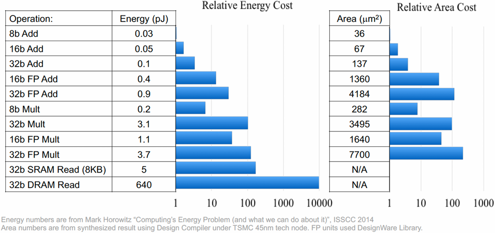
Ampere GPU SM (A100)
Each SM core has:
64 fp32 ALUs (mul-add)
32 int32 ALUs
4 “tensor cores”
Execute 8x4 x 4x8 matrix mul-add instr
A x B + D for matrices A,B,D
A, B stored as fp16, accumulation with fp32 D
There are 108 SM cores in the GA100 GPU:
6,912 fp32 mul-add ALUs
432 tensor cores
1.4 GHz max clock
= 19.5 TFLOPs fp32
+ 312 TFLOPs (fp16/32 mixed) in tensor core
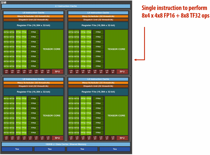
Nvidia H100 GPU (2022)
Fourth-generation Tensor Core
Tensor Memory Accelerator (TMA) unit
CUDA cluster capability
HBM3 with up to 80 GB
TSMC 4nm
80 Billion transistors

Tensor cores

H100 CUDA, Compute and Memory Hierarchies
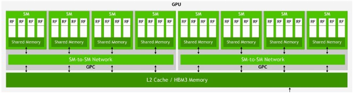
| CUDA Hierarchy | Compute Hierarchy | Memory Hierarchy |
|---|---|---|
| Grid | GPU | 80 GB HBM/ 50 MB L2 |
| Cluster | CPC | 256 KB shared memory per SM |
| Thread Block | SM | 256 KB shared memory |
| Threads | SIMD Lanes | 1 KB RF per thread, 64KB per SM partition |
Thread block cluster is a collective of up to 16 thread blocks
Each thread block is guaranteed to execute on a separate SM and to run at the same time
H100 GPU Streaming Multi-processor (SM)
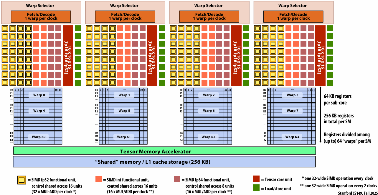
Tensor Memory Accelerator
Special purpose instructions for efficient data movement
Asynchronously load/store a region of a tensor from global to shared memory
Copy descriptor describes region
Single thread issue TMA operation
cuda:memcpy_async
Signal barrier when copy is complete
Hardware address generation and data movement
Copy Descriptor


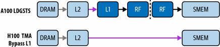
The Whole H100
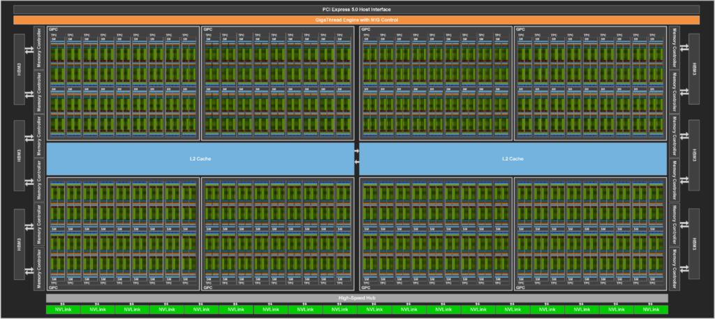
144 SMs
Tensor cores (systolic array MMA): 989 TFLOPS (fp16)
SIMD: 134 TFLOPS (fp16), 67 TFLOPS (fp32)
GPU TFLOPS Over Time
All the TFLOPS are in the Tensor Cores
Nvidia Chips Becoming More Specialized
What are implications for programmers?
V100

A100
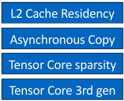
H100
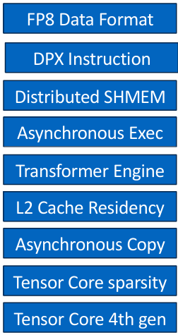
B100
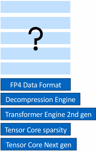
Tensor Cores in B100
Register bandwidth limits for tensor cores in B100
Tensor data in SMEM and TMEM
Single threads execute MMA ⇒ No more warps!
Programming Tensor Cores
Allocate TMEM and descriptors
tcgen05.alloc
Prefetch/stream tiles with TMA (async)
cp.async.bulk.tensor, coordinate with mbarrier
Launch async MMAs
tcgen05.mma batch withtcgen05.commit
Order & retire
tcgen05.fence
Not your father’s CUDA
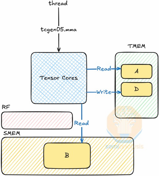
DSLs for GPU AI Kernels
HazyResearch/ThunderKittens: Tile primitives for speedy kernels
CuTe DSL — NVIDIA CUTLASS Documentation
Mojo:面向AI开发者的编程语言 | 强大的CPU和GPU编程 | Mojo官网 Mojo社区 – Mojo
Pallas:Mosaic GPU — JAX 文档
How Ideal are GPUs
| Feature | Why? | Nvidia GPU |
|---|---|---|
| Tiled tensors (e.g. 16 x 16, 32 x 32) | Max TFLOPS on GEMM Low instr. overhead | ✅ |
| Asynchronous compute | Overlap compute and memory access | ✅ mma_async |
| Asynchronous memory access | Overlap compute and memory access | ✅ TMA+TMEM |
| Asynchronous chip-to-chip communication | Overlap compute, memory and communication | |
| Compute unit to compute unit comm. | Fusion and pipelining Streaming Dataflow | ❓ TB Cluster |
Hardware acceleration of AI inference/training

Google’s TPU (v1)
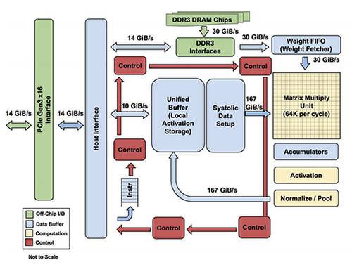
TPU area proportionality(比例)
Arithmetic units ~ 30% of chip
Note low area footprint of control
Key instructions:
read host memory
write host memory
read weights
matrix_multiply / convolve
activate
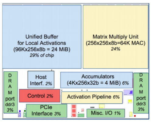
Floor Plan of TPU die(yellow = compute, blue = data, green = I/O, red = control)
Systolic array
(matrix vector multiplication example: y=Wx)
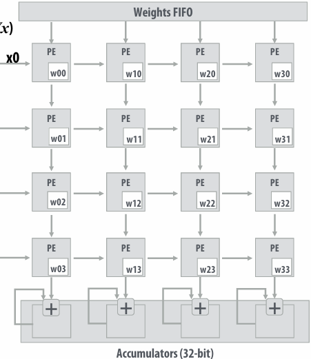
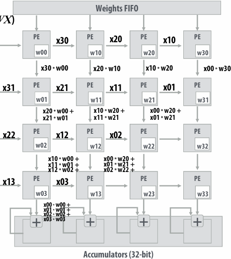
Notice: need multiple 4x32bit accumulators to hold output columns
Systolic Array Dataflow
| Dataflow Type | What stays in each PE | What streams through | Main goal |
|---|---|---|---|
| Weight-Stationary (WS) | Weight values | Inputs (activations) and partial sums | Minimize reloading of weights |
| Output-Stationary (OS) | Partial sums (outputs) | Inputs and weights | Minimize movement of accumulated results |
| Input-Stationary (IS) | Input activations | Weights and partial sums | Minimize reloading of inputs |
SIMD vs. Systolic Array
| Feature | SIMD | Systolic Array |
|---|---|---|
| Dataflow | Control-driven (instructions) | Data-driven (wavefront) |
| Locality (data reuse) | Limited | Temporal and spatial |
| Communication | Global (register/memory) | Local (neighbor PEs) |
| Control | Centralized | Distributed |
| Efficiency (perf/mm2, perf/Watt) | Medium | Very high |
Building larger matrix-matrix multiplies
Example: A = 8x8, B= 8x4096, C=8x4096
Assume 4096 accumulators
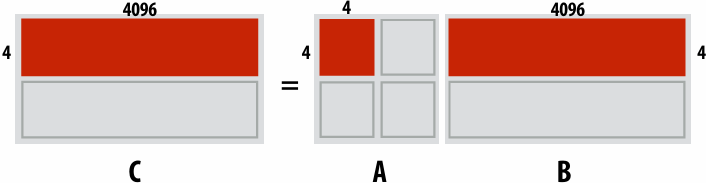
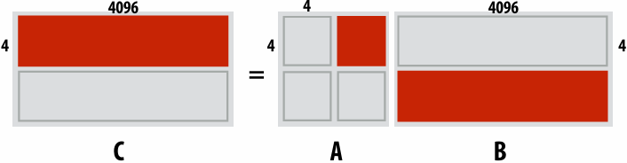
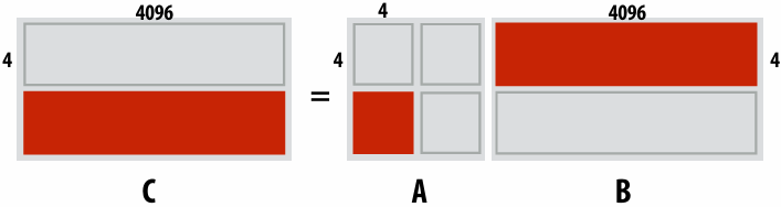
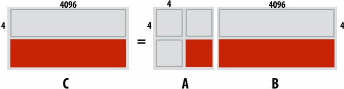
TPU Performance/Watt
GM = geometric mean over all apps total = cost of host machine + CPU
WM = weighted mean over all apps incremental = only cost of TPU
Evolution of Google TPUs
Hardware Lottery
When a research idea wins because it is suited to the available software and hardware and not because the idea is universally superior to alternative research directions
AI Models ⇒ Dataflow Architecture
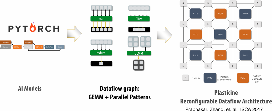
Reconfigurable Dataflow Architecture vs Ideal Accelerator
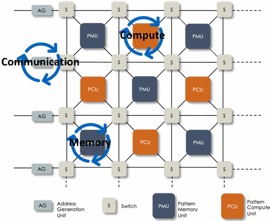
No instructions ⇒ No instruction fetch/decode overhead
Extreme asynchrony: no sequential instruction execution
Dataflow Kernel Fusion
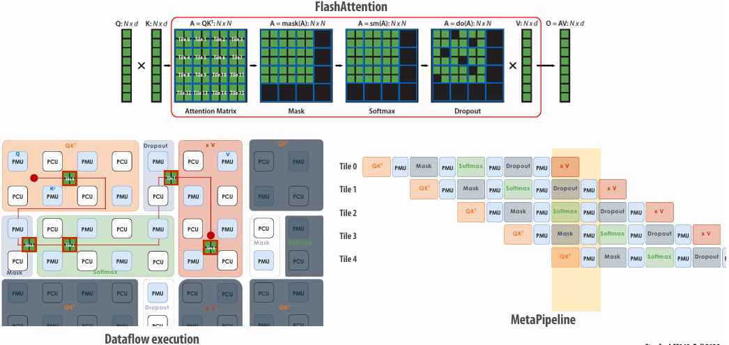
Summary: specialized hardware for AI model processing
Specialized hardware for executing key DNN computations efficiently
Feature many arithmetic units
Customized/configurable datapaths to directly move intermediate data values between processing units (schedule computation by laying it out spatially on the chip) at multiple granularities
Large amounts of on-chip storage for fast access to intermediates
Lecture 11: Programming Specialized Hardware for AI
Specialization Improves Efficiency
Tensor Cores
Specialized MMA compute
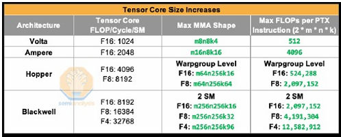
Warpgroup: 128 consecutive threads
PTX: Parallel Thread Execution
NVIDIA’s virtual instruction set architecture
TMA
Specialized block data movement unit
Eliminates 1000’s of instructions and memory addressing overhead
Eliminates unnecessary data movement through L1 and registers
GPU Kernels are Important
2025 GPU market is enormous ⇒ NVIDIA 2025 quarterly revenue of > $47B
GPU AI kernels are often run on clusters of hundreds of millions of dollars of GPUs, for months on end. (e.g. large training runs, serving models at scale, etc.)
FlashAttention-2 degraded from ~70% on A100s to ~35% on H100s. Took 2 years to come back up to ~65% with FlashAttention-3
Poor kernels underutilize billions of dollars worth of compute
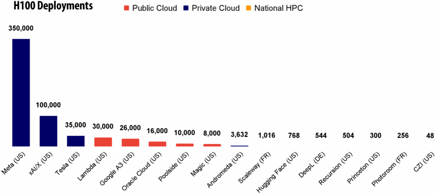
Extracting Peak Performance from the H100
Kernels that keep the Tensor cores busy (>90% of TFLOPS)
Use 16 x 16 tiles of fp16 data ⇒ matches Tensor core compute
Make sure compute is never idle
Overlap memory access and compute ⇒ use asynchrony
A tile processing pipeline
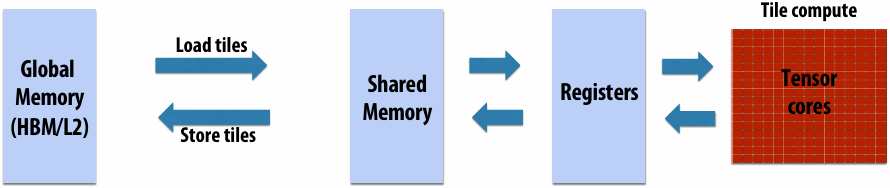
ThunderKittens
A Simple Embedded DSL for AI kernels
Design principle #1: tile of 16x16 as primitive data type
TK manages layouts
TK provides basic operations
Design principle #2: Asynchrony, everywhere
Expose primitives for user to manage, if top performance needed
Design principle #3: High-level GPU coordination patterns
Producer-consumer processing
Embedded CUDA DSL template library
Templated Data Types
Register tiles: 2D tensors on the register file
height, width, and layout
Register vectors: 1D tensors on the register file
length and layout
Shared memory tiles: 2D tensors in shared memory
height, width, and layout
Shared memory vectors: 1D tensors in shared memory
Length
Operations
Initializers – zero out a shared vector, for example
Unary ops, like exp
Binary ops, like mul
Row / column ops, like a row_sum
Tile Processing Pipeline with ThunderKittens
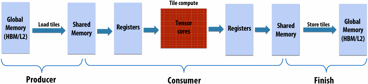
TK Matmul
Step 1: Define layouts
1 |
|
Step 2: Define pipeline and producers
1 | struct matmul_template { |
Step 3: Compute!
1 | struct consumer { |
TK Matmul Performance
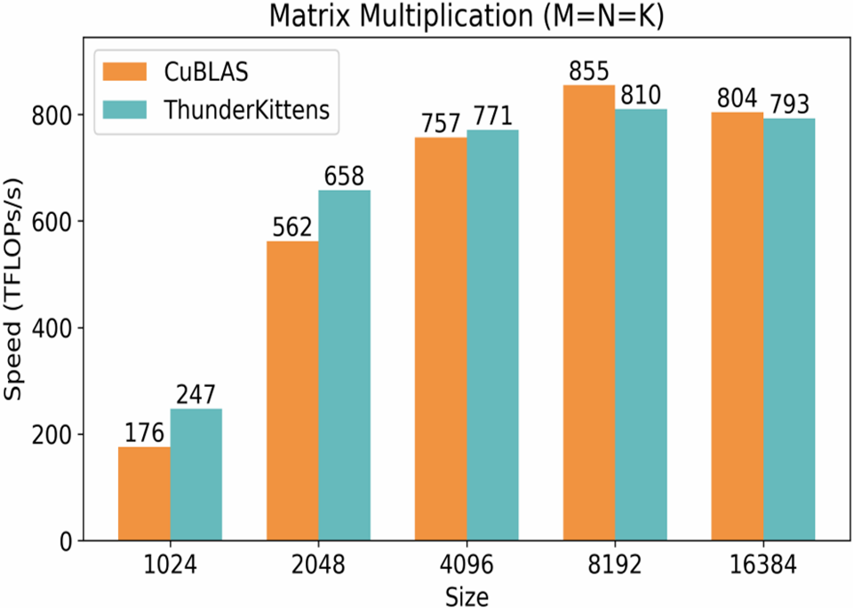
Metapipelining
Can we have asynchrony with a simpler programming model? (Hint: Take a data-centric view)
Recall: AI Models are Dataflow Graphs
AI Models ⇒ Dataflow Architecture
Streaming Dataflow ⇒ Kernel Fusion
Attention Algorithm
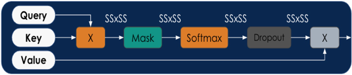
Attention Algorithm on RDA
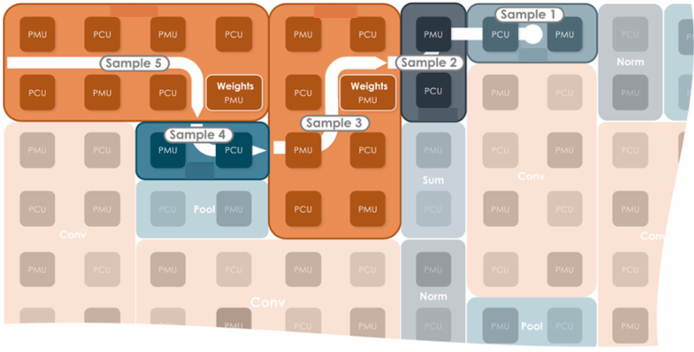
Coarse -grained pipelining
Reconfigurable Dataflow
SambaNova SN40L RDU
1,040 PCUs and PMUs
638 TFLOPS (bf16)
520 MB on-chip SRAM
64 GB HBM
1.5 TB DDR
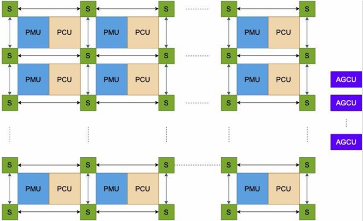
PCU: Pattern Compute Unit
systolic and SIMD compute (16 x 8 bf16)
PMU: Pattern Memory Unit
High address generation flexibility and bandwidth (0.5 MB)
S: Mesh switches
High on-chip interconnect flexibility and bandwidth
AGCU: Address Generator and Coalescing Unit
Portal to off-chip memory and IO
Dataflow Programming with Data Parallel Patterns
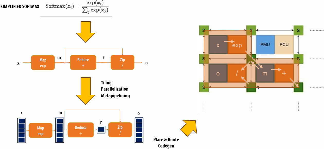
Composable Compute Primitives: MM, Map, Zip, Reduce, Gather, Scatter …
Flexible scheduling in space and time ⇒ spatial execution
Metapipelining
Hierarchical coarse-grained pipeline: A “pipeline of pipelines”
Exploits nested-loop parallelism
Convert parallel pattern (loop) into a streaming pipeline
Insert pipe stages in the body of the loop
Pipe stages execute in parallel
Overlap execution of multiple loop iterations
Intermediate data between stages stored in double buffers
Handles imbalanced stages with varying execution times
Tiling and fusion
Works well with tiling
Buffers can be used to change access pattern (e.g. transpose data)
Metapipelining can work when fusion does not
Metapipelining Intuition
Gaussian Discriminant Analysis (GDA)
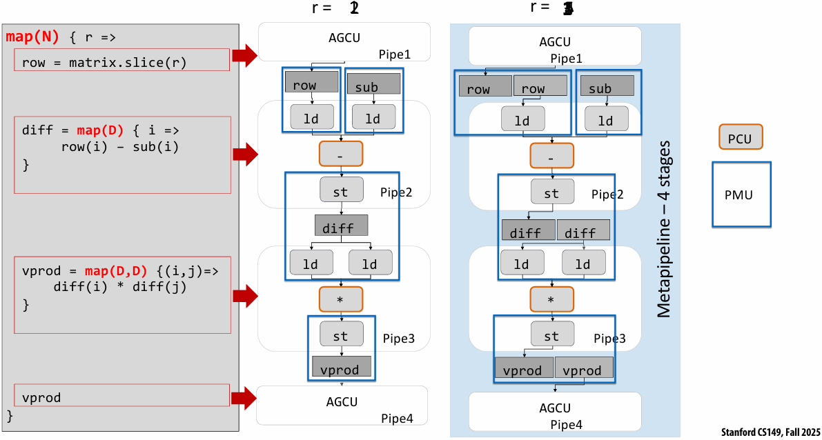
Matmul Metapipeline
1 | auto format = DataFormat::kBF16; |
Matmul Metapipe
1 | METAPIPE(M, MM) { |
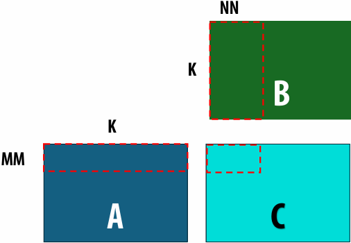
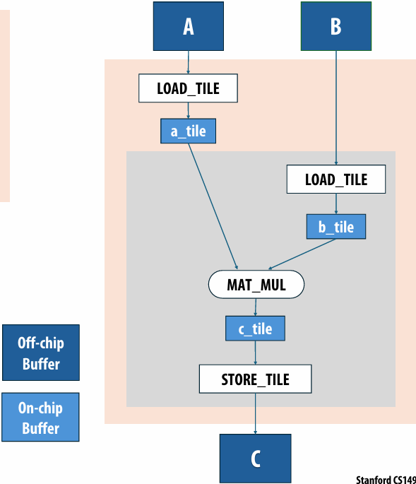
Matmul Metapipe Mapping
FlashAttention Metapipeline
FlashAttention
Dataflow execution with token control ⇒ no lock-based synchronization
MetaPipeline = Streaming Dataflow
Llama3.1 8B
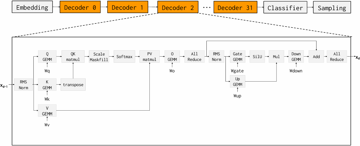
Limited Kernel Fusion on GPUs
Llama3.1 8B with Tensor-RT LLM
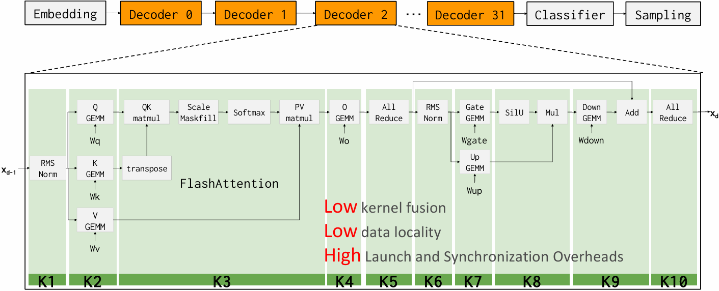
RDU Fuses Entire Decoder into One Kernel !
Llama3.1 8B with aggressive kernel fusion
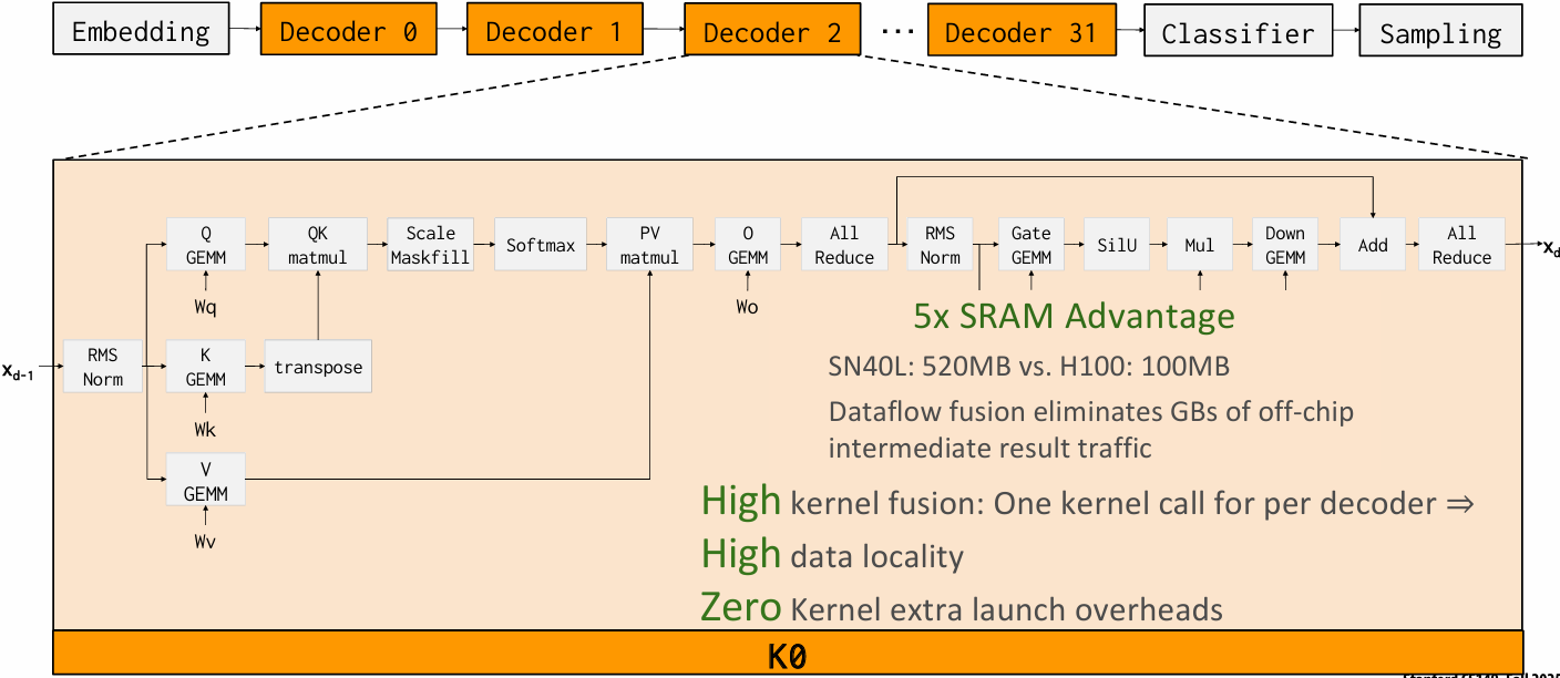
Kernel Loop
Asynchronous memory and compute
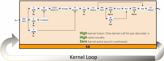
One kernel call for all decoders
3 calls per token on RDU
~800 calls per token on GPU
100x fewer kernel calls
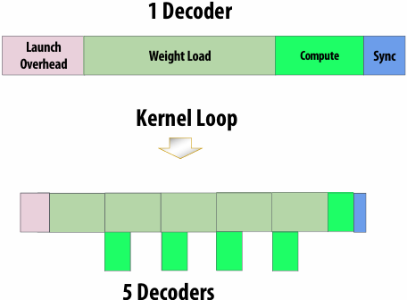
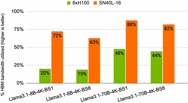
Dataflow ⇒ High Performance
Overlap compute, memory access, chip-to-chip communication
Fully overlap allreduce with weight load and compute
Allreduce does not consume HBM capacity or bandwidth
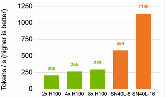
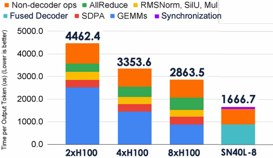
Summary: SpecializedHardware and Programming for AI Models
Specialized hardware for executing key AI computations efficiently
Feature large/many matrix multiply units implemented with systolic arrays
Customized/configurable datapaths to directly move intermediate data values between processing units (schedule computation by laying it out spatially on the chip)
Large amounts of on-chip storage for fast access to intermediates
H100: Asynchronous compute and memory mechanisms ⇒ complex programming
Need ThunderKittens and other DSLS to manage complexity
SN40L: Dataflow model with metapipelining ⇒ simpler programming model
Sophisticated compiler to optimize and map to dataflow hardware
Minimizing synchronization overheads required for high performance
Lecture 12: Mapping AI Applications to the AI Datacenter
Short Primer on Memory
CPU vs GPU Memory
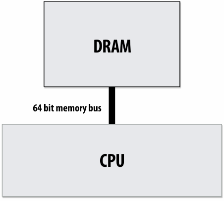
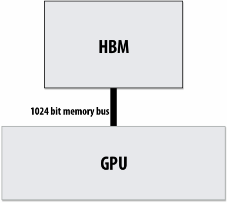
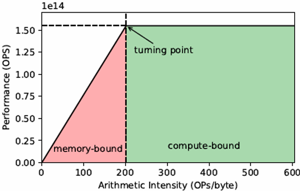
Increase bandwidth, reduce power by chip stacking
Enabling technology: 3D stacking of DRAM chips
DRAMs connected via through-silicon-vias (TSVs) that run through the chips
TSVs provide highly parallel connection between logic layer and DRAMs
Base layer of stack “logic layer” is memory controller, manages requests from processor
Silicon “interposer(中介)” serves as high-bandwidth interconnect between DRAM stack and processor
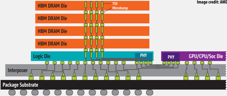
Technologies:
Micron/Intel Hybrid Memory Cube (HBC)
High-bandwidth memory (HBM) - 1024 bit interface to stack
HBM Advantages
More Bandwidth
High Power Efficiency
Small Form Factor
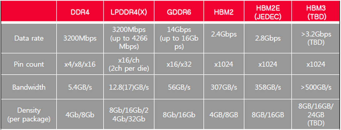
GPUs are adopting HBM technologies
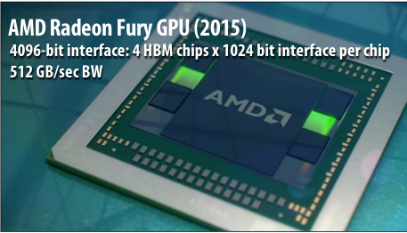
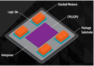
NVIDIA P100 GPU (2016)
4096-bit interface: 4 HBM2 chips x 1024 bit interface per chip
720 GB/sec peak BW
4 x 4 GB = 16 GB capacity
NVIDIA H100 GPU (2022)
6144-bit interface: 6 HBM3 stacks x 1024 bit interface per stack
3.2 TB/sec peak BW
80 GB capacity
Nvidia HBM Roadmap
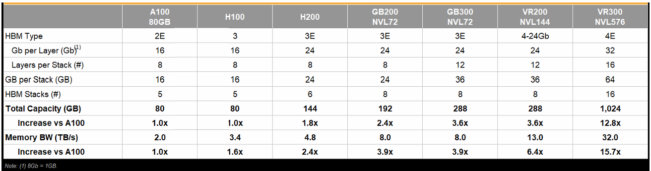
AI Cluster Size

Scale Up and Scale Out
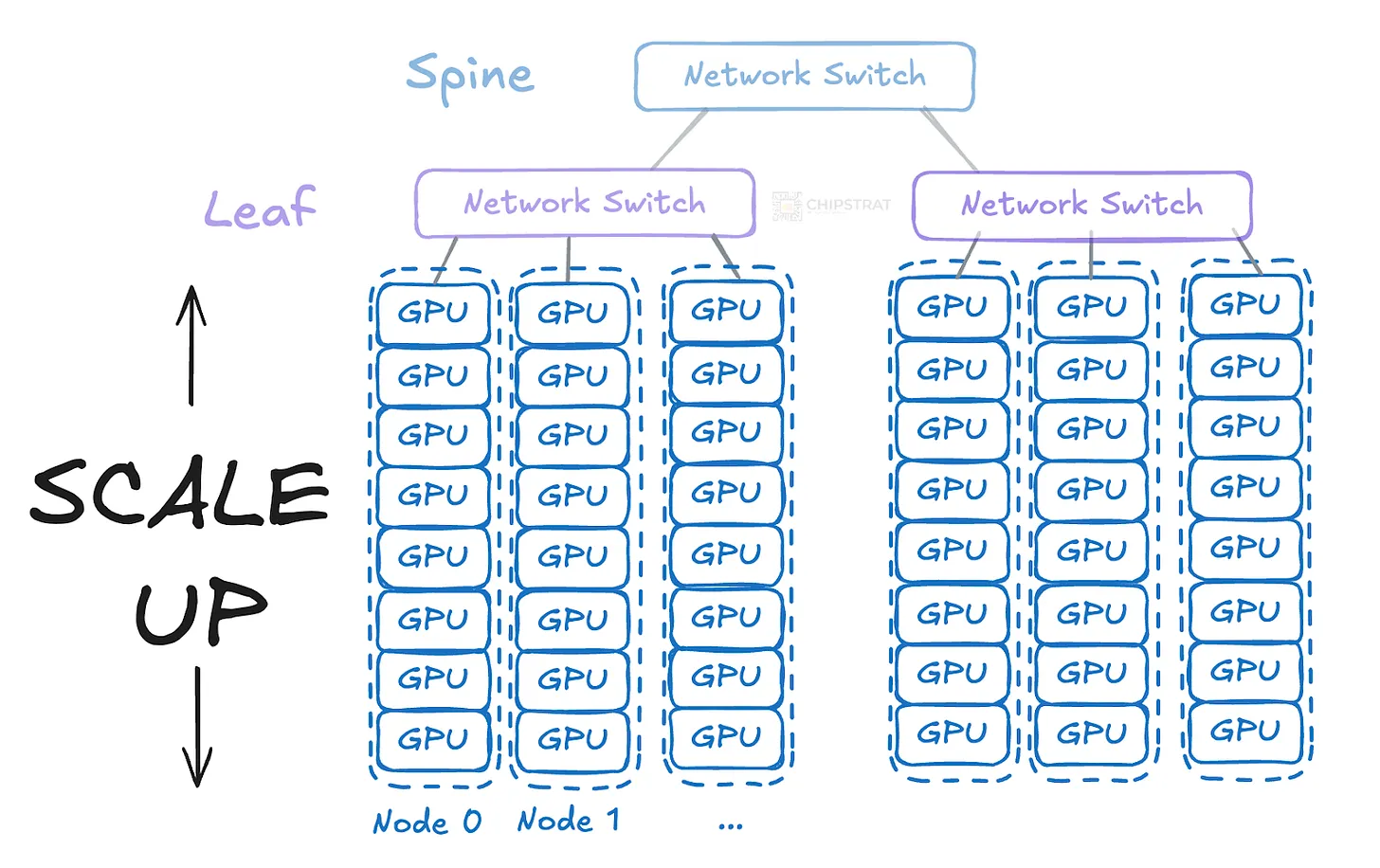
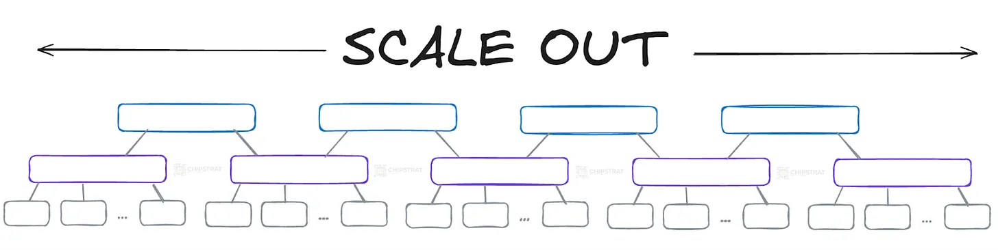
DGX SUPERPOD
Modular Architecture
1K GPU SuperPOD Cluster
140 DGX A100 nodes (1,120 GPUs) in a GPU POD
1st tier fast storage - DDN AI400x with Lustre
Mellanox HDR 200Gb/s InfiniBand - Full Fat-tree
Network optimized for AI and HPC
DGX A100 Nodes
2x AMD 7742 EPYC CPUs + 8x A100 GPUs
NVLINK 3.0 Fully Connected Switch
8 Compute + 2 Storage HDR IB Ports
A Fast Interconnect
Modular IB Fat-tree
Separate network for Compute vs Storage
Adaptive routing and SharpV2 support for offload
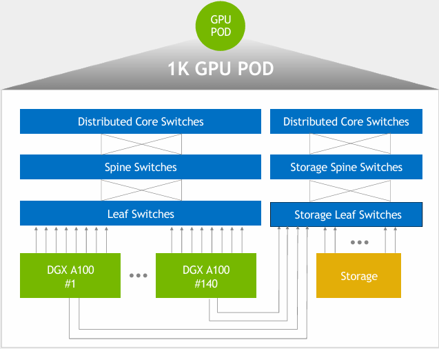
Message Passing Communication Primitives: AllReduce, ReduceScatter, AllGather
rank = accelerator node
Collective Operations — NCCL 2.29.1 documentation
AllReduce
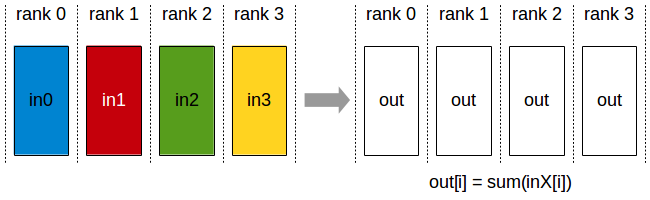
ReduceScatter
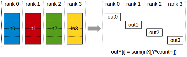
AllGather
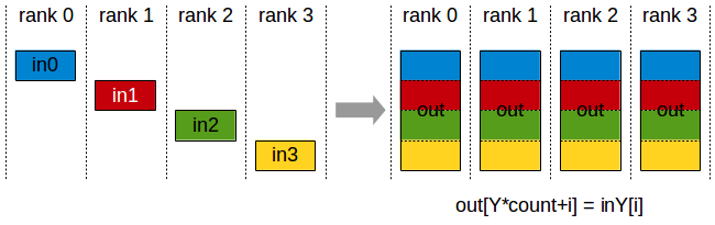
Message Passing Communication Primitives: All-to-All
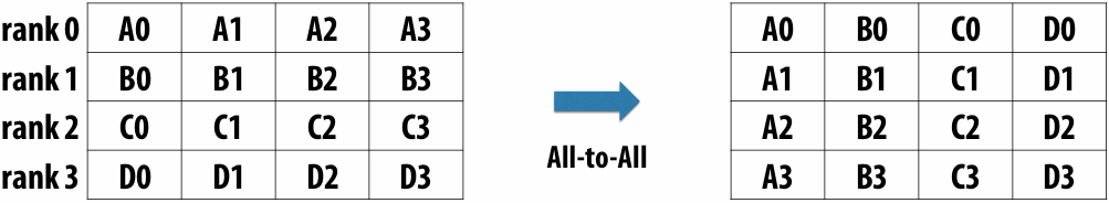
Transformer
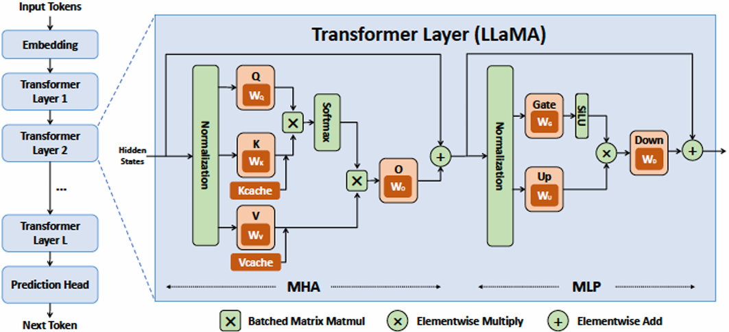
Where is the Parallelism in AI Models?
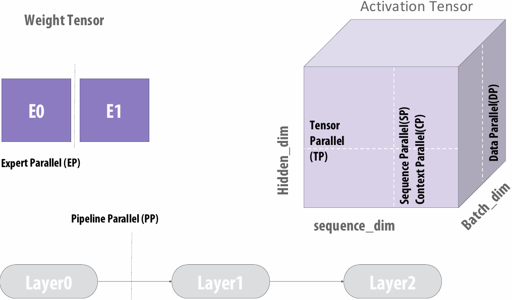
Parallelism and Communication
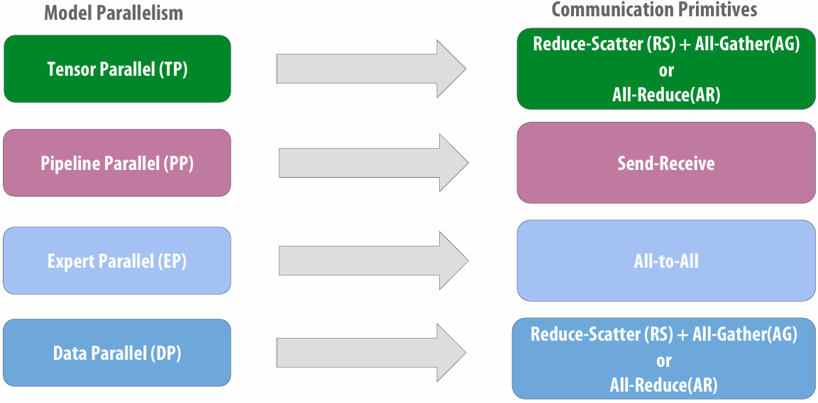
Distributed Matrix-Multiply Example
inputA[MxK] * inputB[KxN] = out[MxN]
BS = 16, M = 24576, K = 131072, N = 8192
Mapping: Distribute K dimension across S RDUs
Matrix multiply size per socket: [MxK/S] * [K/SxN] = [MxN]
Produces S partial results of size [MxN], one per socket
S-way reduce-scatter to combine the partial results
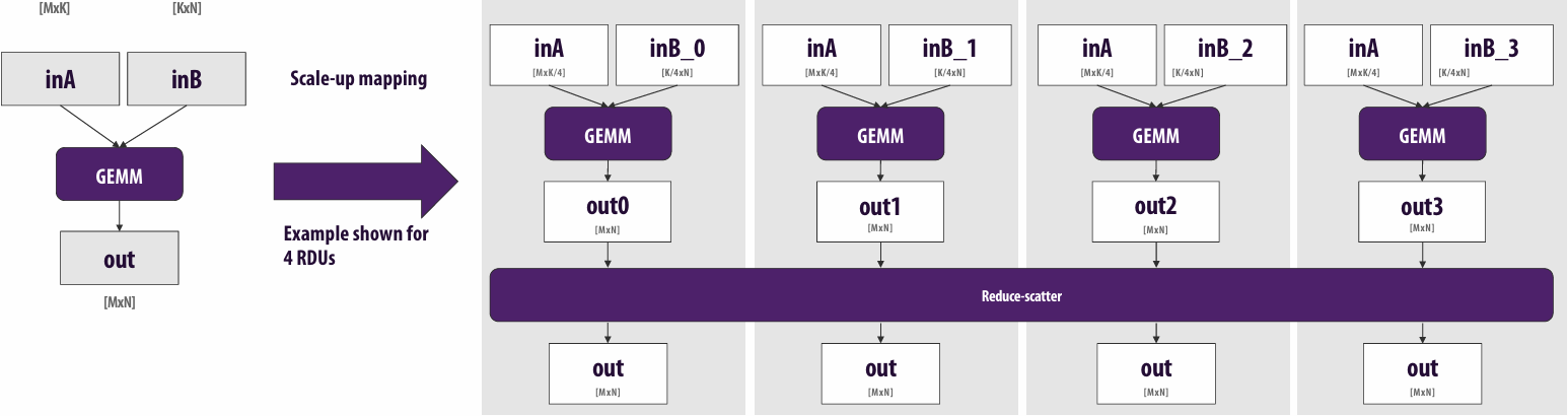
Compute - Communication Overlap
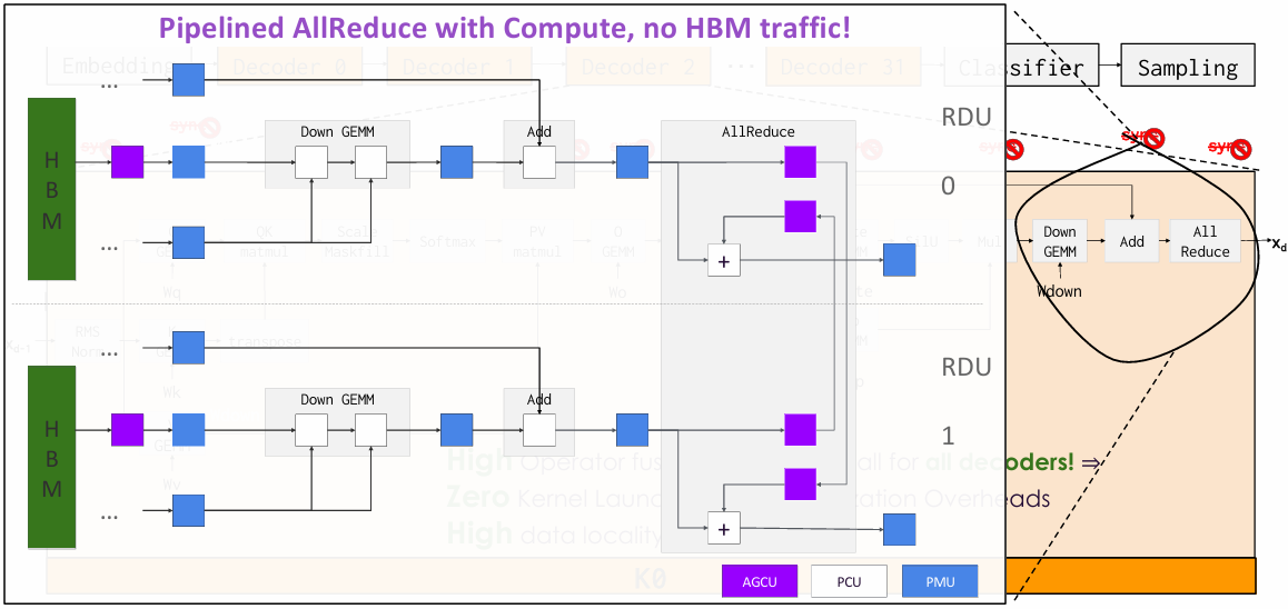
Importance of Overlap - Conceptual
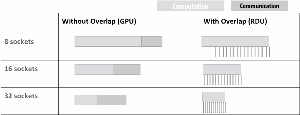
Communication time increases on GPUs with more sockets
Communication becomes the bottleneck without overlap
GPUs need need large interconnect bandwidth to get high utilization
Importance of Overlap - Quantified on RDUs
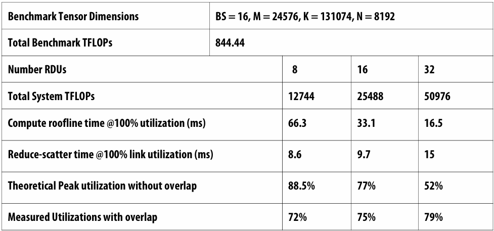
Sustained 70+% utilization across 32 sockets due to compute-communication overlap
Pipeline Parallelism and Training
Under-utiliization of compute resources
Low overall throughput
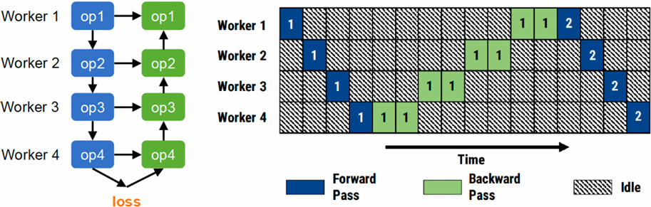
Fine-grained Pipeline Parallelism
Mini-batch: the number of samples processed in each iteration
Divide a mini-batch into multiple micro-batches
Pipeline the forward and backward computations across micro-batches
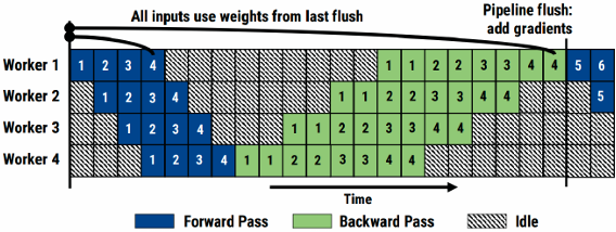
Tensor, Data, Pipeline Parallelism
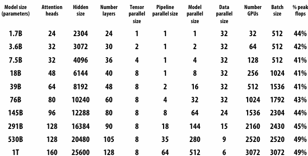
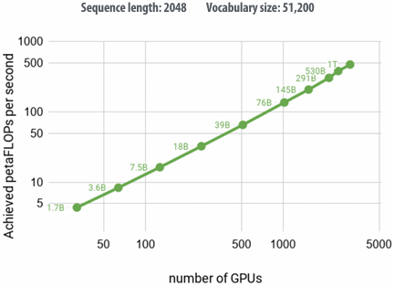
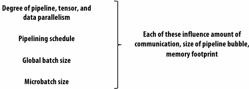
Accessing Memory (a basic tutorial on how DRAM works)
Reducing energy consumption idea 1: use specialized processing (use the right processor for the job)
Reducing energy consumption idea 2: move less data
Data Access has high energy cost
Rule of thumb in mobile system design: always seek to reduce amount of data transferred from memory
Earlier in class we discussed minimizing communication to reduce stalls (poor performance)
Now, we wish to reduce communication to reduce energy consumption
“Ballpark” numbers http://www.displaymate.com/iPad_ShootOut_1.htm
Integer op: ~ 1 pJ (Cost to just perform the logical operation, not counting overhead of instruction decode, load data from registers, etc.)
Floating point op: ~20 pJ (Cost to just perform the logical operation, not counting overhead of instruction decode, load data from registers, etc.)
Reading 64 bits from small local SRAM (1mm away on chip): ~ 26 pJ
Reading 64 bits from low power mobile DRAM (LPDDR): ~1200 pJ (Suggests that recomputing values, rather than storing and reloading them, is a better answer when optimizing code for energy efficiency!)
Implications
Reading 10 GB/sec from memory: ~1.6 watts
Entire power budget for mobile GPU: ~1 watt (remember phone is also running CPU, display, radios, etc.)
iPhone 16 battery: ~14watt-hours (note: my MacbookPro laptop: 99 watt-hour battery)
Exploiting locality matters!!!
Moving data is costly!
Data movement limits performance
Many processing elements…
= higher overall rate of memory requests
= need for more memory bandwidth
(result: bandwidth-limited execution)
Data movement has high energy cost
~ 0.9 pJ for a 32-bit floating-point math op
~ 5 pJfor a local SRAM (on chip) data access
~ 640 pJto load 32 bits from LPDDR memory
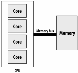
The memory system
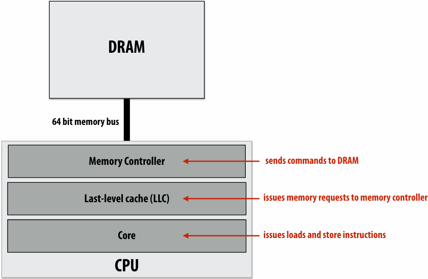
DRAM array
1 transistor(晶体管) + capacitor(电容器) per “bit” (recall from physics: a capacitor stores charge)
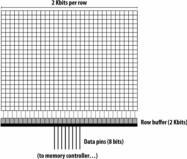
DRAM operation (load one byte)
Estimated latencies are in units of memory clocks: DDR3-1600 (Kayvon’s laptop at the time of making this slide)
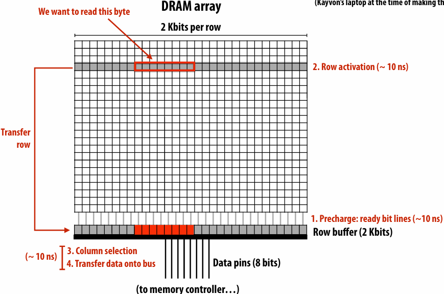
Load next byte from (already active) row
Lower latency operation: can skip precharge and row activation steps
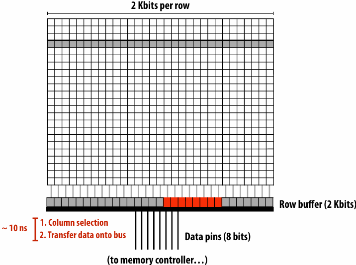
DRAM access latency is not fixed
Best case latency: read from active row
Column access time (CAS)
Worst case latency: bit lines not ready, read from new row
Precharge (PRE) + row activate (RAS) + column access (CAS)
Precharge readies bit lines and writes row buffer’s contents back into DRAM array (reading a row is destructive)
Question 1: when to execute precharge?
After each column access
Only when new row is accessed?
Question 2: how to handle latency of DRAM access?
Problem: low pin utilization due to latency of access
Data pins in use only a small fraction of time (red = data pins busy)
This is bad since they are the scarcest(最稀有的) resource!
DRAM burst mode
Idea: amortize latency over larger transfers
Each DRAM command describes bulk transfer
Bits placed on output pins in consecutive clocks
DRAM chip consists of multiple banks
All banks share same pins (only one transfer at a time)
Banks allow for pipelining of memory requests
Precharge/activate rows/send column address to one bank while transferring data from another
Achieves high data pin utilization
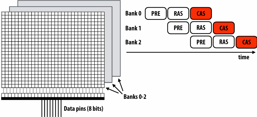
Organize multiple chips into a DIMM
Example: Eight DRAM chips (64-bit memory bus)
Note: DIMM appears as a single, higher capacity, wider interface DRAM module to the memory controller. Higher aggregate bandwidth, but minimum transfer granularity is now 64 bits
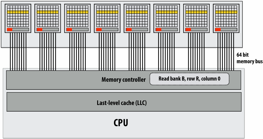
Reading one 64-byte (512 bit) cache line (the wrong way)
Assume: consecutive physical addresses mapped to same row of same chip
Memory controller converts physical address to DRAM bank, row, column
All data for cache line serviced by the same chip
Bytes sent consecutively over same pins (8 bits per clock —> cache line takes 64 cycles to transfer!)
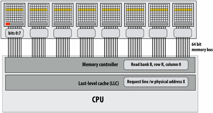
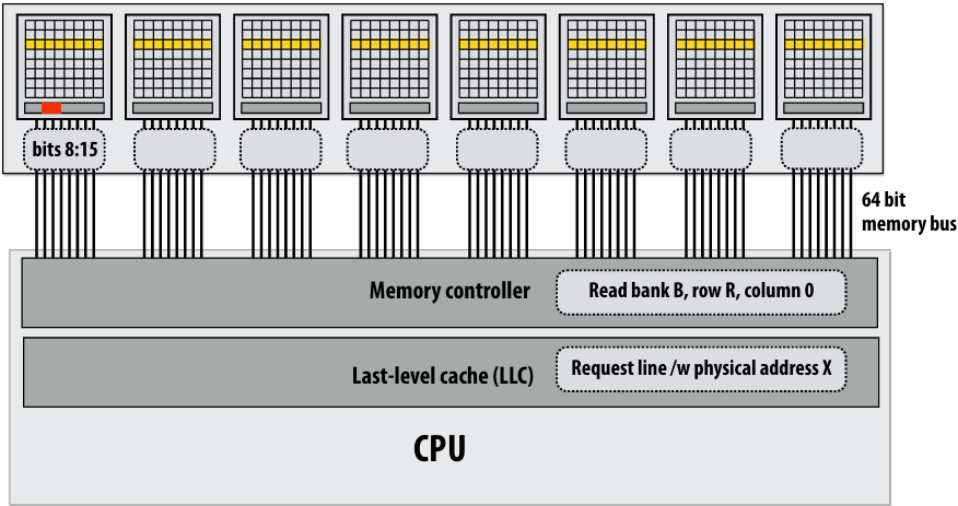

Reading one 64-byte (512 bit) cache line (efficient way)
Memory controller converts physical address to DRAM bank, row, column
Here: physical addresses are interleaved across DRAM chips at byte granularity
DRAM chips transmit first 64 bits in parallel (cache line takes 8 clocks to transfer)
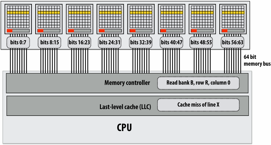
DRAM controller requests data from new column (Recall modern DRAM’s support burst mode transfer of multiple consecutive columns, which would be used here)
DRAM chips transmit next 64 bits in parallel
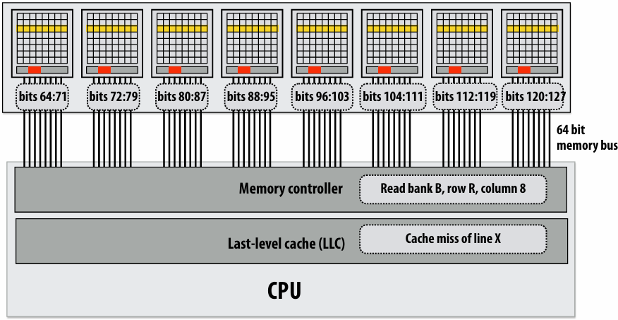
Memory controller is a scheduler of memory requests
Receives load/store requests from LLC
Conflicting scheduling goals
Maximize throughput, minimize latency, minimize energy consumption
Common scheduling policy: FR-FCFS (first-ready, first-come-first-serve)
Service requests to currently open row first (maximize row locality)
Service requests to other rows in FIFO order
Controller may coalesce(合并) multiple small requests into large contiguous requests (to take advantage of DRAM “burst modes”)
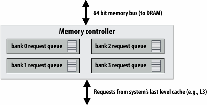
Dual-channel memory system
Increase throughput by adding memory channels (effectively widen memory bus)
Below: each channel can issue independent commands
Different row/column is read in each channel
Simpler setup: use single controller to drive same command to multiple channels
Example: DDR4 memory
Processor: Intel® Core™ i7-7700K Processor (in Myth cluster)
Memory system details from Intel’s site:
Intel® Core™ i7-7700K Processor
DDR4 2400
64-bit memory bus x 1.2GHz x 2 transfers per clock(DDR stands for “double data rate”) = 19.2 GB/s per channel
2 channels = 38.4 GB/sec
~13 nanosecond CAS
DRAM summary
DRAM access latency can depend on many low-level factors
Discussed today:
State of DRAM chip: row hit/miss? is recharge necessary?
Buffering/reordering of requests in memory controller
Significant amount of complexity in a modern multi-core processor has moved into the design of memory controller
Responsible for scheduling ten’s to hundreds of outstanding memory requests
Responsible for mapping physical addresses to the geometry of DRAMs
Area of active computer architecture research
Modern architecture challenge:
improving memory performance:
Decrease distance data must move by locating memory closer to processors (enables shorter, but wider interfaces)
Increase bandwidth, reduce power by chip stacking
Enabling technology: 3D stacking of DRAM chips
DRAMs connected via through-silicon-vias (TSVs) that run through the chips
TSVs provide highly parallel connection between logic layer and DRAMs
Base layer of stack “logic layer” is memory controller, manages requests from processor
Silicon “interposer(中介)” serves as high-bandwidth interconnect between DRAM stack and processor
Technologies:
Micron/Intel Hybrid Memory Cube (HBC)
High-bandwidth memory (HBM) - 1024 bit interface to stack
HBM Advantages
More Bandwidth
High Power Efficiency
Small Form Factor
GPUs are adopting HBM technologies
NVIDIA P100 GPU (2016)
4096-bit interface: 4 HBM2 chips x 1024 bit interface per chip
720 GB/sec peak BW
4 x 4 GB = 16 GB capacity
NVIDIA H100 GPU (2022)
6144-bit interface: 6 HBM3 stacks x 1024 bit interface per stack
3.2 TB/sec peak BW
80 GB capacity
HBM4 Custom Logic Die
Xeon Phi (Knights Landing) MCDRAM
16 GB in package stacked DRAM
Can be treated as a 16 GB last level cache
Or as a 16 GB separate address space (“flat mode”)
Intel’s claims:
~ same latency at DDR4
~5x bandwidth of DDR4
~5x less energy cost per bit transferred
1 | // allocate buffer in MCDRAM (“high bandwidth” memory malloc) |
The memory bottleneck is being addressed in many ways
By the application programmer
Schedule computation to maximize locality, increase arithmetic intensity (minimize required data movement)
By new hardware architectures
Intelligent DRAM request scheduling
Bringing data closer to processor (deep cache hierarchies, 3D stacking)
Increase bandwidth (wider memory systems)
Ongoing research in locating limited forms of computation “in” or near memory
Ongoing research in hardware accelerated compression(压缩) (not discussed today)
General design principles
Locate data storage near processor
Move computation to data storage
Data compression (trade-off extra computation for less data transfer)
Three trends in energy-optimized computing
Compute less!
Computing costs energy: parallel algorithms that do more work than sequential counterparts may not be desirable even if they run faster
Specialize compute units:
Heterogeneous processors: CPU-like cores + throughput-optimized cores (GPU-like cores)
Fixed-function units: audio processing, “movement sensor processing” video decode/encode, image processing/computer vision?
Specialized instructions: expanding set of AVX vector instructions, new instructions for accelerating AES encryption (AES-NI)
Programmable soft logic: FPGAs
Reduce bandwidth requirements
Exploit locality (restructure algorithms to reuse on-chip data as much as possible)
Aggressive use of compression: perform extra computation to compress application data before transferring to memory (likely to see fixed-function HW to reduce overhead of general data compression/decompression)
【2023】Lecture 17: Hardware Specialization and Algorithm Specific Programming
Challenges of heterogeneous designs:
(it’s not easy to realize the potential of specialized, heterogeneous processing)
Heterogeneous system: preferred processor for each task
Challenge to software developer: how to map application onto a heterogeneous collection of resources?
Challenge: “Pick the right tool for the job”: design algorithms that decompose into components that each map well to different processing components of the machine
The scheduling problem is more complex on a heterogeneous system
Challenge for hardware designer: what is the right mixture of resources?
Too few throughput oriented resources (lower peak throughput for parallel workloads)
Too few sequential processing resources (limited by sequential part of workload)
How much chip area should be dedicated to a specific function, like video?
Summary: heterogeneous processing for efficiency
Heterogeneous parallel processing: use a mixture of computing resources that fit mixture of needs of target applications
Latency-optimized sequential cores, throughput-optimized parallel cores, domain-specialized fixed-function processors
Examples exist throughout modern computing: mobile processors, servers, supercomputers
Traditional rule of thumb in “good system design” is to design simple, general-purpose components
This is not the case in emerging systems (optimized for perf/watt)
Today: want collection of components that meet perf requirement AND minimize energy use
Challenge of using these resources effectively is pushed up to the programmer
Current CS research challenge: how to write efficient, portable programs for emerging heterogeneous architectures?
Spatial
Mapping Algorithms to Execution Resources
General Purpose Processor
Special Purpose Processor (Accelerator)
So You Want to Design an Accelerator for Your Algorithm
Traditionally, you must spend years becoming an expert in VHDL or Verilog, Chisel…
High-Level Synthesis (HLS): Vivado HLS, Intel OpenCL, and Xilinx SDAccel
Restricted C with pragmas
These tools sacrifice performance and are difficult to use
Spatial is a high-level language for designing hardware accelerators that was designed to enable performance-oriented programmers to specify
Parallelism: specialized compute
Locality: specialized memories and data movement
Spatial: DSL for Accelerator Design
Simplify configurable accelerator design
Constructs to express:
Parallel patterns as parallel and pipelined datapaths
Independent parallelism
Dependent parallelism
hierarchical control
explicit memory hierarchies
Explicit parameters
All parameters exposed to the compiler
Simple APIs to manage CPU ⇔ Accelerator communication
Allows programmers to focus on “interesting stuff”
Designed for performance-oriented programmers (parallelism and locality)
More intuitive than CUDA: dataflow instead of threads
The Spatial Language: Memory Templates
1 | // Explicit memory hierarchy |
The Spatial Language: Control Templates
1 | // Blocking/non-blocking interaction with CPU |
The Spatial Language: Design Parameters
Spatial templates capture a variety of design parameters:
1 | // Explicit parallelization factors |
Inner Product
Let’s build an accelerator to see how Spatial works
Inner Product in C
Here is inner product written in C for a CPU
1 | // Set up accumulator and memory pointers |
Inner Product in Spatial
Inner product in Spatial allows the programmer to build a hardware accelerator
Start of code looks like C example
Accel instantiates “for” loop in hardware
1 | // Set up host and memory pointers |
1 | // Set up host and memory pointers |
Spatial generates multi-step controllers (This Reduce controller’s final step will handle the accumulation)
1 | // Set up host and memory pointers |
Spatial manages communication with DRAM
1 | // Set up host and memory pointers |
1 | // Set up host and memory pointers |
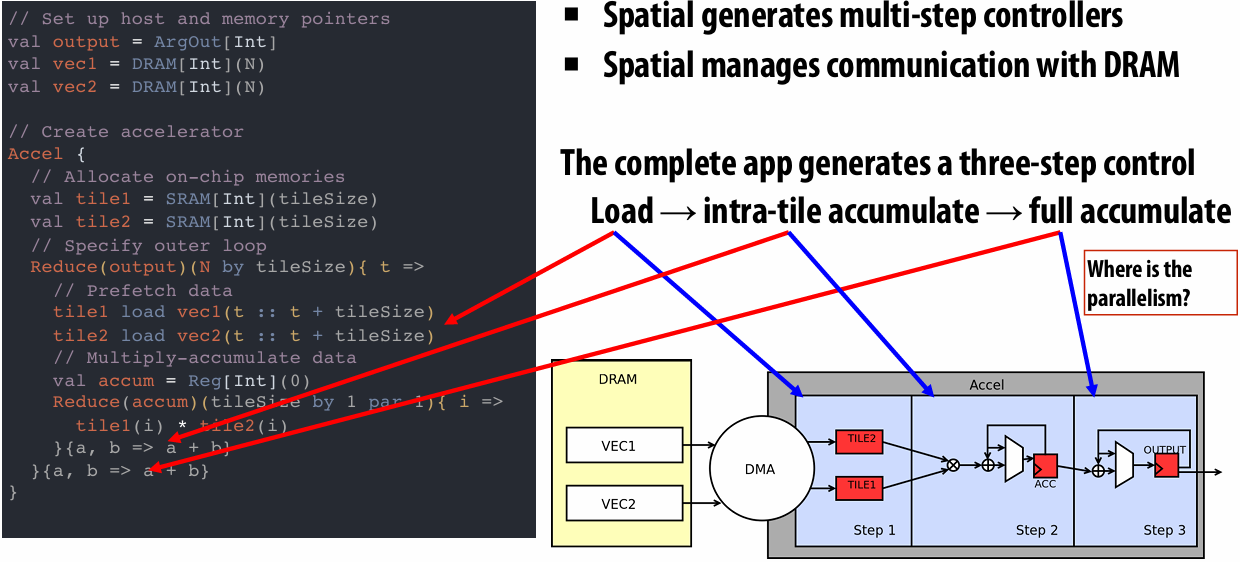
pipeline that, so that that’s one place that we could exploit parallelism in a product representation
parallelize step 2, SIMD would be a good way of parallelizing step 2 since we’re doing the same operation to all of the elements in the tile
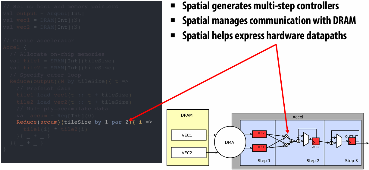
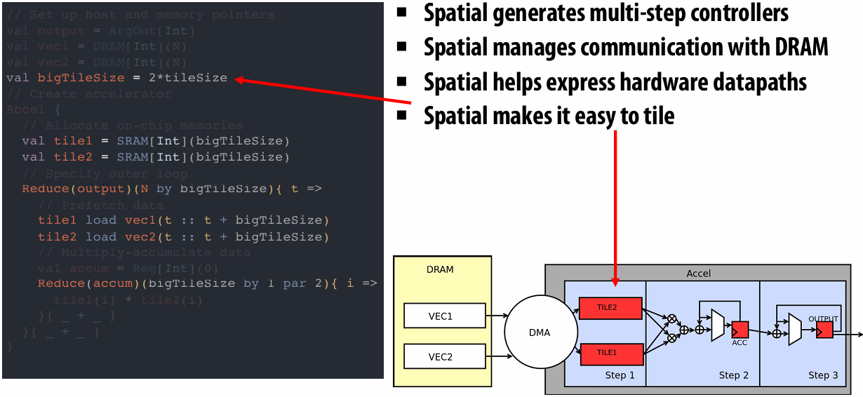
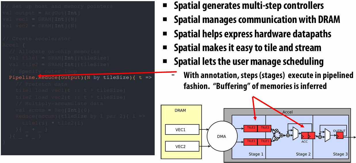
Spatial Question
Spatial programmer’s responsibility
Specifying algorithm as a hierarchy of controllers
Specifying memory hierarchy of algorithm
Explicit data movement
Picking tiling factors, parallelism and scheduling
Spatial compiler’s responsibility
Banking and buffering of memories to maximize perf and minimize resources
Hardware generation for target platform (FPGA, CGRA, ASIC)
Performance debugging feedback
TensorFlow to FPGA
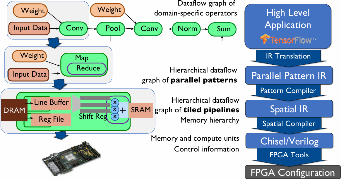
Kernel versus Stream Execution
Recap: Why was Flash Attention powerful?
Fused attention
for each j:
for each i:
Load block Qi, KTj, Vj, Oi
Compute Sij = QiKTj
Compute Mij = m(Sij), Pij = f(Sij), and lij = l(Sij) (all functions operate row-wise on row-vectors)
Multiply PijVj and accumulate into Oi with appropriate scalings
Save memory footprint: Never materialize N2 matrix
Save memory bandwidth: (high arithmetic intensity)
Read 3 blocks (from Q, K, V)
Do two matrix multiplies + a few row summations
Accumulate into O block (which is resident in cache)
Note there is additional computation vs. the original version (must re-scale prior values of O each step of i-loop)
With streaming execution, we get these benefits for free! (Free Fusion!)
Streaming execution model: Free Fusion!
Kernel-based Execution Model:
FlashAttention prevents the materialization of the N x N matrix
However, it requires modifying the algorithm and extra computation
Streaming execution model:
Avoids materialization of the N x N matrix
Without algorithmic changes & extra computation
Preliminary: Softmax
Softmax is actually a 3-step operation
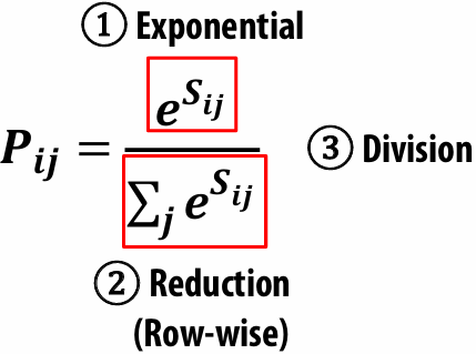
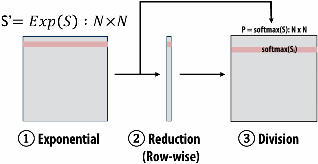
Attention
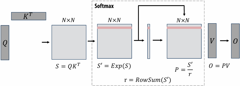
Kernel-based Execution Model
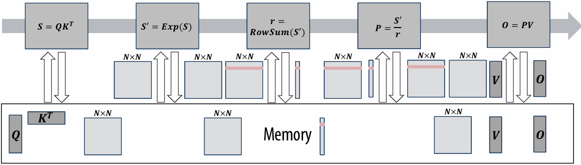
Materialize the N x N matrix ⇒ ↑ Memory Footprint
Read & write the N x N matrix ⇒ ↑ Memory bandwidth
Streaming Execution Model
With the streaming execution model, we get fusion for free which means:
Avoid materializing the N x N matrix ⇒ ↓ Memory Footprint
Avoid reading & writing the intermediate N x N matrices ⇒ ↓ Memory bandwidth
An example program in a streaming execution model
Computation: Exponential & Rowsum
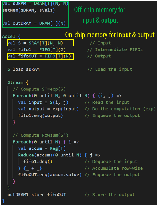
Doing the computation piece-wise
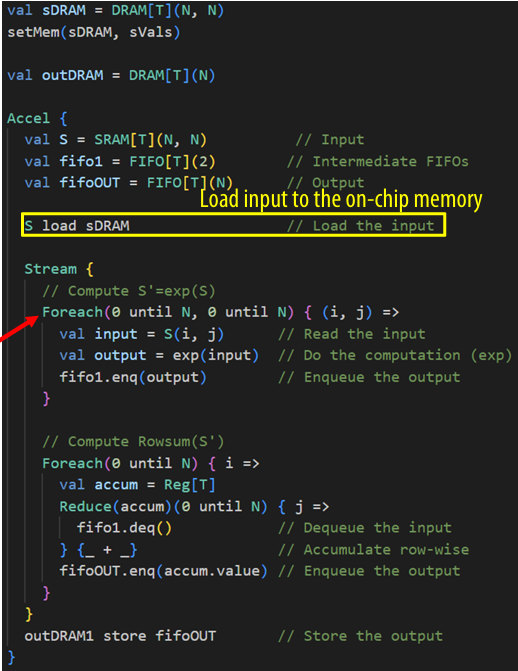
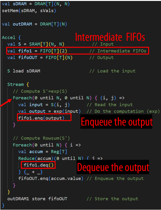
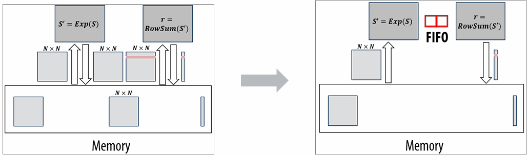
Kernel-based Execution Model (Overview)
Streaming Execution Model (Overview)
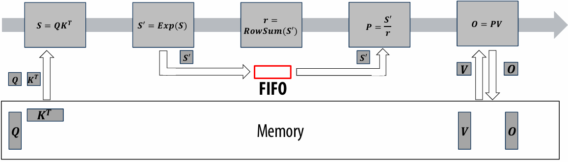
Streaming Execution Model
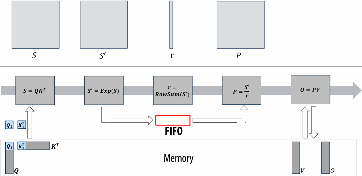
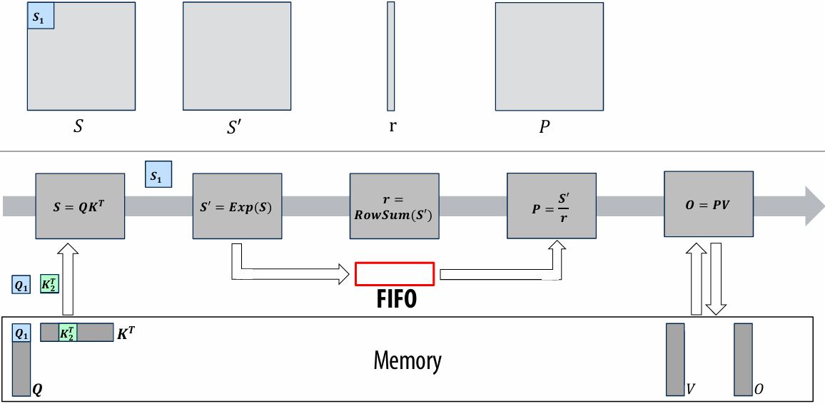
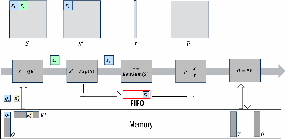
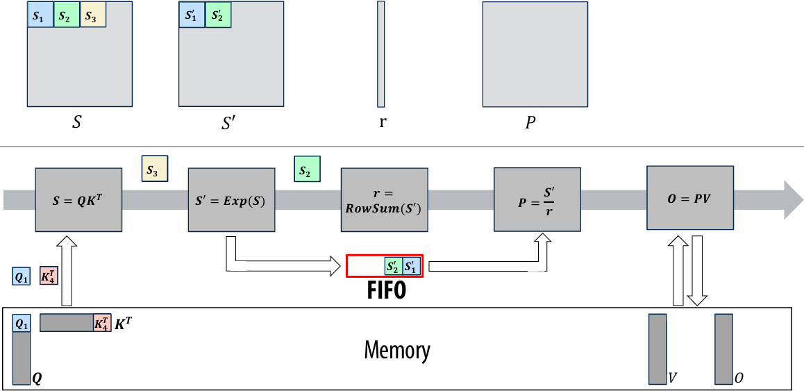
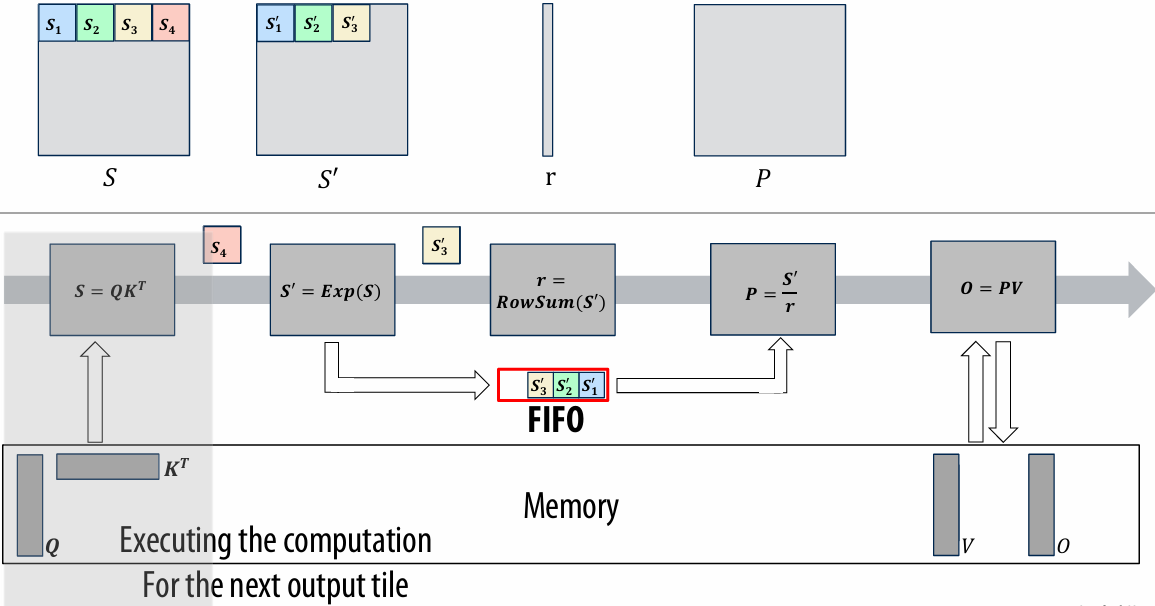
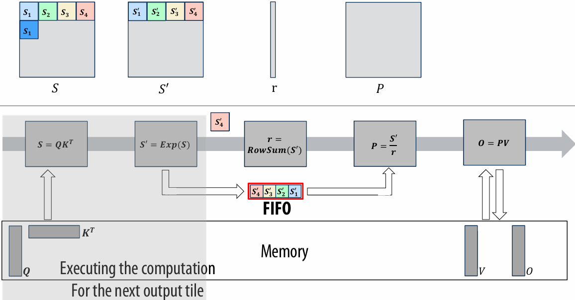
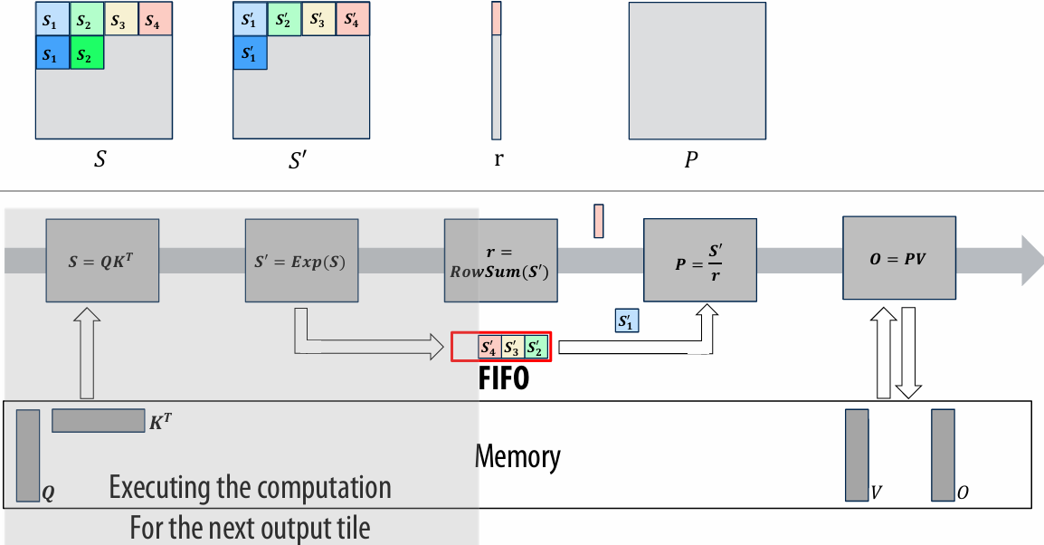
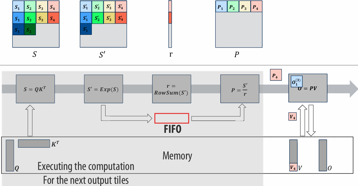
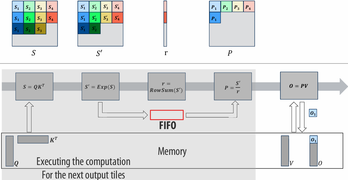
Can we do better with FlashAttention?
Yes!
By paying a bit more computation cost as Flash Attention does, we can eliminate the FIFO in the middle
We needed this sequence-length (N) sized FIFO to buffer the output of 𝑆= 𝐸𝑥𝑝(𝑆)
This is because in softmax, we have to wait until the row-wise reduction (row sum) is calculated to divide the output of 𝑆= 𝐸𝑥𝑝(𝑆) with the row sum
Flash Attention breaks this dependency by:
Reordering operations
Using a running sum & rescaling instead of the naïve reduction (row sum)
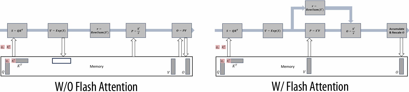
Kernel versus Stream Execution
More parallelism
FlashAttention with kernel-based execution model:
Cannot overlap the computation for different output tiles
Streaming execution model
Spatially maps each computation with pipeline communication
Can overlap (pipeline) the computation for different output tiles!
Don’t have to manually create fused kernels
FlashAttention with kernel-based execution model:
Have to manually write fused kernels in CUDA
Often challenging to fuse deeply due to the limit in (# of registers / SM)
Streaming execution model
Operations gets fused automatically if we write the program using FIFOs
Compiler can automatically generate fused executioin
Accelerator Design Summary
Significant energy efficiency improvements from specialized accelerators (100x–1000x)
Designing an accelerator is a tradeoff between performance and resource utilization
Parallelism
Locality
It requires the programmer to have insight into the application
Where is the bottleneck
Is the implementation compute or memory-bound
Spatial helps you understand the trade-off between performance and resource utilization
Allows rapid exploration of your algorithm
Enables high-level accelerator design
Lecture 13: Domain-Specific Programming Systems and Automatic Performance Optimization
Domain specific languages
Performance optimization in languages like C++, ISPC, CUDA = low productivity (Proof by assignments 1, 2, 3, 4, etc…)
The ideal parallel programming language
Popular languages (not exhaustive ;-))
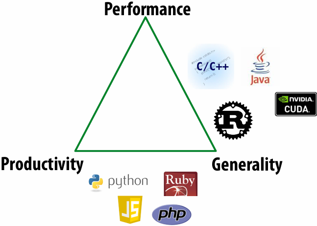
Way forward ⇒ domain-specific languages
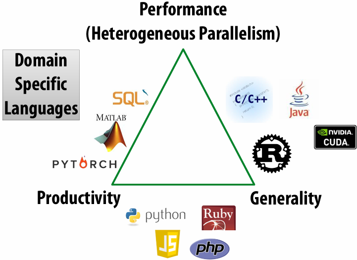
Domain specific languages
Domain Specific Languages (DSLs)
Programming language with restricted expressiveness for a particular domain
High-level, usually declarative, and deterministic
Domain-specific programming systems
Main idea: raise level of abstraction for expressing programs
Goal: quickly write a high-performance program for a target machine
Goal: write one program, and run it efficiently on different machines
Introduce high-level programming primitives specific to an application domain
Productive: intuitive(直观) to use, portable(可移植的) across machines, primitives correspond to behaviors frequently used to solve problems in targeted domain
Performant: system uses domain knowledge to provide efficient, optimized implementation(s)
Given a machine: system knows what algorithms to use, parallelization strategies to employ for this domain
Optimization goes beyond efficient mapping of software to hardware! The hardware platform itself can be optimized to the abstractions as well
Cost: loss of generality/completeness
A DSL example: Halide: a domain-specific language for image processing
Jonathan Ragan-Kelley, Andrew Adams et al. [SIGGRAPH 2012, PLDI 13]
Halide used in practice
Halide used to implement camera processing pipelines on Google phones
HDR+, aspects of portrait(人像) mode, etc…
Industry usage at Instagram, Adobe, etc.
3x3 image blur
Total work per image = 9 x WIDTH x HEIGHT
For NxN lter: N2 x WIDTH x HEIGHT
1 | int WIDTH = 1024; |
Two-pass 3x3 blur
A 2D separable lter (such as a box lter) can be evaluated via two 1D ltering operations
Total work per image = 6 x WIDTH x HEIGHT
For NxN lter: 2N x WIDTH x HEIGHT
WIDTH x HEIGHT extra storage
2x lower arithmetic intensity than 2D blur (2x memory access)
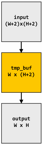
1 | int WIDTH = 1024; |
Two-pass image blur: locality
Intrinsic bandwidth requirements of blur algorithm:
Application must read each element of input image and must write each element of output image
1 | int WIDTH = 1024; |
Two-pass image blur, “chunked” (version 1)
Total work per row of output:
step 1: 3 x 3 x WIDTH work
step 2: 3 x WIDTH work
Total work per image = 12 x WIDTH x HEIGHT
Loads from tmp_buffer are cached (assuming tmp_buffer fits in cache)
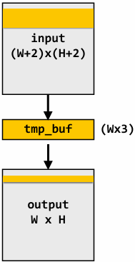
1 | int WIDTH = 1024; |
Two-pass image blur, “chunked” (version 2)
Total work per chuck of output: (assume CHUNK_SIZE = 16)
Step 1: 18 x 3 x WIDTH work
Step 2: 16 x 3 x WIDTH work
Total work per image: (34/16) x 3 x WIDTH x HEIGHT = 6.4 x WIDTH x HEIGHT
Trends to ideal value of 6 x WIDTH x HEIGHT as CHUNK_SIZE is increased!
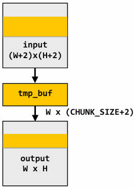
1 | int WIDTH = 1024; |
Still not done
We have not parallelized loops for multi-core execution
We have not used SIMD instructions to execute loops bodies
Other basic optimizations: loop unrolling, etc…
Optimized C++ code: 3x3 image blur
Good: ~10x faster on a quad-core CPU than my original two-pass code
Bad: specific to SSE (not AVX2), CPU-code only, hard to tell what is going on at all!
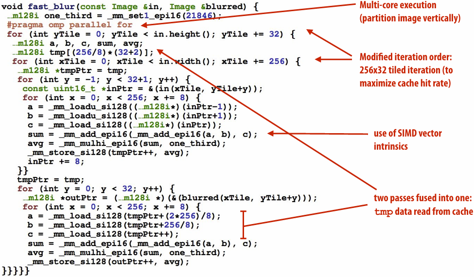
Halide language
Simple domain-specific language embedded in C++ for describing sequences of image processing operations
Halide function: an infinite(无限) (but discrete(离散)) set of values defined on N-D domain
Halide expression: a side-effect free expression that describes how to compute a function’s value at a point in its domain in terms of the values of other functions
1 | Var x, y; |
Image processing application as a DAG
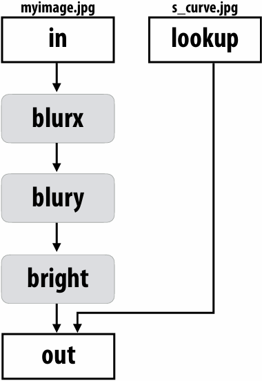
Key aspects of representation
Intuitive expression:
Adopts local “point wise” view of expressing algorithms
Halide language is declarative. It does not define order of iteration, or what values in domain are stored!
It only defines what is needed to compute these values
Iteration over domain points is implicit (no explicit loops)
1 | Var x, y; |
One (serial) implementation of Halide
1 | Equivalent “C-style” loop nest: |
Key aspect in the design of any system: Choosing the “right” representations for the job
Good representations are productive to use:
Embody(体现) the natural way of thinking about a problem
Good representations enable the system to provide the application useful services:
Validating/providing certain guarantees (correctness, resource bounds, conversation of quantities, type checking)
Performance (parallelization, vectorization, use of specialized hardware)
Now the job is not expressing an image processing computation, but generating an efficient implementation of a specific Halide program
A second set of representations for “scheduling”
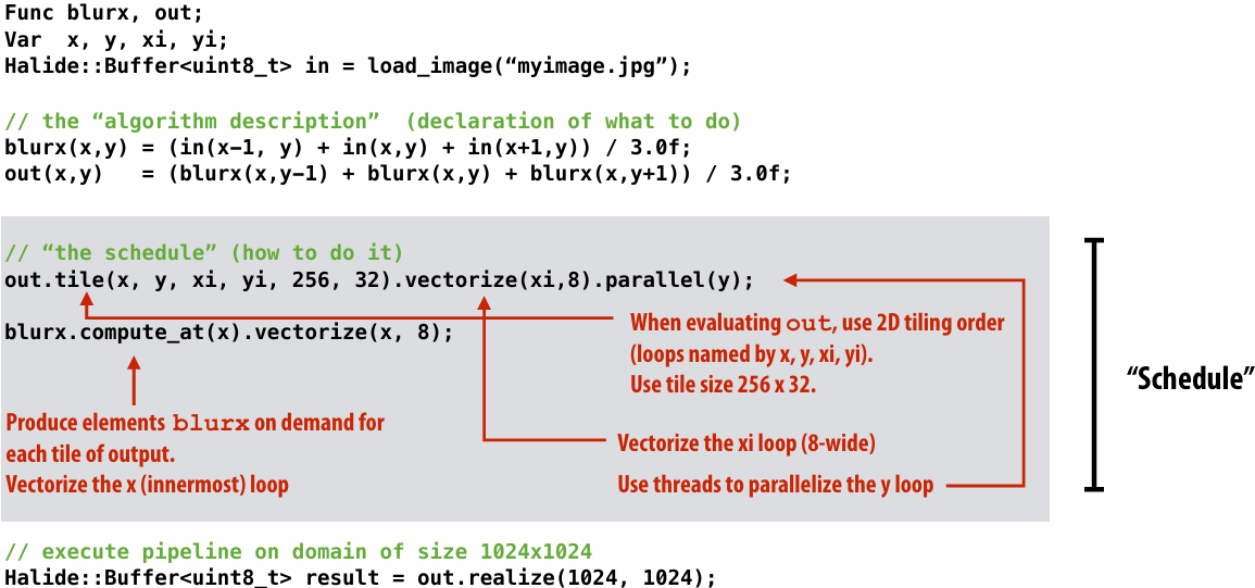
Scheduling primitives allow the programmer to specify a high-level “sketch” of how to schedule the algorithm onto a parallel machine, but leave the details of emitting the low-level platform-specific code to the Halide compiler
Primitives for iterating over N-D domains
Specify both order and how to parallelize (multi-thread, vectorize via SIMD instr)
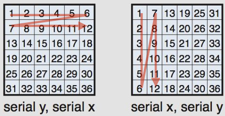
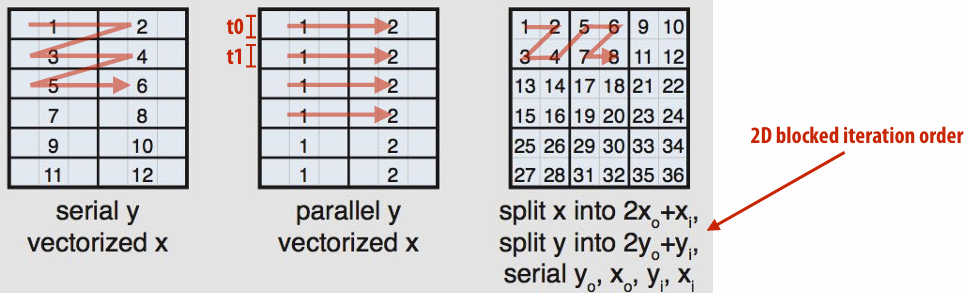
(In diagram, numbers indicate sequential order of processing within a thread)
Specifying loop iteration order and parallelism
1 | blurx(x,y) = (in(x-1, y) + in(x,y) + in(x+1,y)) / 3.0f; |
Primitives for how to interleave producer/consumer processing
1 | // Halide algorithm: |
Loop nest diagram of implementation:
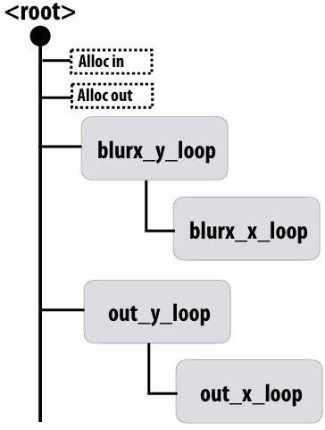
1 | // Halide algorithm: |
Loop nest diagram of implementation:
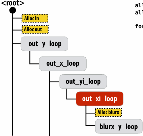
1 | // Halide algorithm: |
Loop nest diagram of implementation:
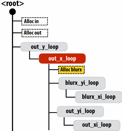
Summary of scheduling the 3x3 box blur
1 | // the “algorithm description” (declaration of what to do) |
What is the philosophy(理念) of Halide?
Programmer is responsible for describing an image processing algorithm
Programmer has knowledge of how to schedule the application efficiently on machine (but it’s slow and tedious), so Halide gives programmer a second language to express high-level scheduling decisions
Loop structure of code
Unrolling / vectorization / multi-core parallelization
The system (Halide compiler) is not smart, it provides the service of mechanically(机械地) carrying out the details of the schedule in terms of mechanisms available on the target machine (phthreads, AVX intrinsics, etc.)
Constraints on language (to enable compiler to provide desired services)
Application domain scope: computation on regular N-D domains
Only feed-forward(前馈) pipelines (+ special support for reductions and fixed depth recursion(递归) )
All dependencies inferable(推断) by compiler
Initial academic Halide results
Application 1: camera RAW processing pipeline (Convert RAW sensor data to RGB image)
Original: 463 lines of hand-tuned ARM NEON assembly
Halide: 2.75x less code, 5% faster
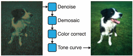
Application 2: bilateral(双边) filter (Common image filtering operation used in many applications)
Original 122 lines of C++
Halide: 34 lines algorithm + 6 lines schedule
CPU implementation: 5.9x faster
GPU implementation: 2x faster than hand-written CUDA
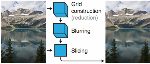
Stepping back: what is Halide?
Halide is a DSL for helping expert developers optimize image processing code more rapidly
Halide does not decide how to optimize a program for a novice(新手) programmer
Halide provides primitives for a programmer (that has strong knowledge of code optimization) to rapidly express what optimizations the system should apply
Halide compiler carries out the nitty-gritty(细节) of mapping that strategy to a machine
Automatically generating Halide schedules
Problem: it turned out that very few programmers have the ability to write good Halide schedules
80+ programmers at Google write Halide
Very small number trusted to write schedules
Solution: extend compiler to analyze Halide program to automatically generate efficient schedules for the programmer [Adams 2019]
As of [Adams 2019], you’d have to work pretty hard to manually author a schedule that is better than the schedule generated by the Halide autoscheduler for image processing applications
See “Learning to Optimize Halide with Tree Search and Random Programs”, Adams et al. SIGGRAPH 2019
Modeling scheduling as a sequence of choices
For each node N in the program DAG, starting from the end of the DAG…
Choose where to place current node N in the existing loop nest (determine N.compute_at())
Choose a tile sizes for N (assume outer dimension is parallel over threads, inner dimension is vectorized)
Repeat until entire DAG is scheduled
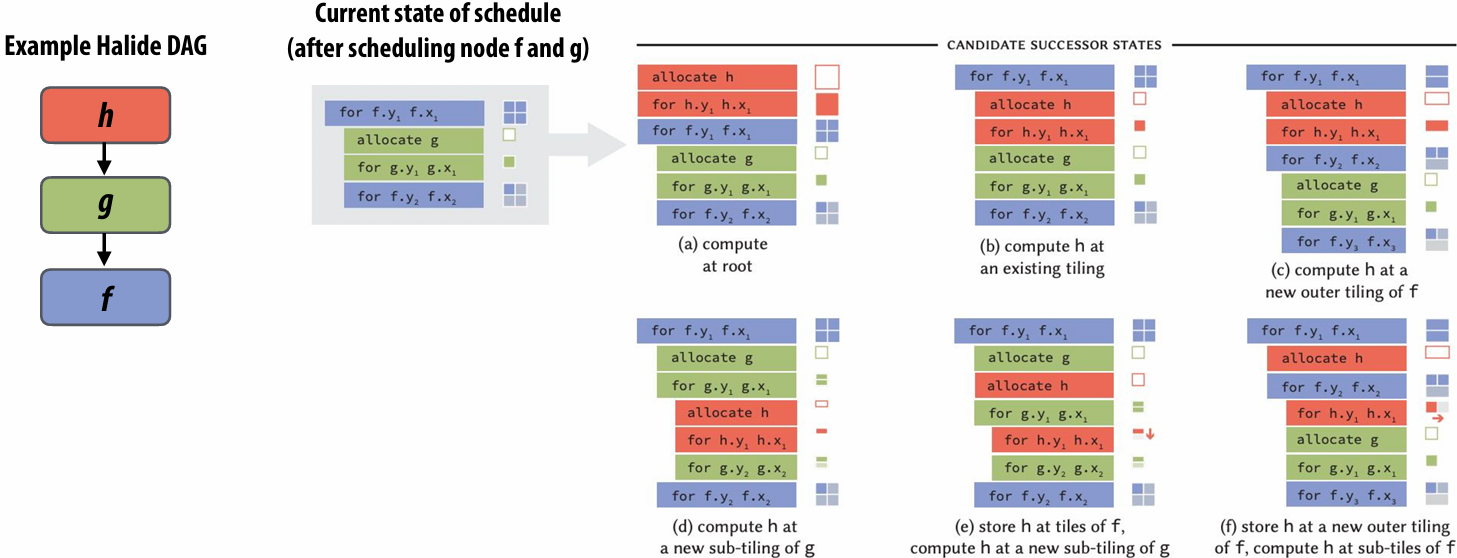
Use search to find best performing schedule
Search over large space of schedules (e.g., greedy search, beam search)
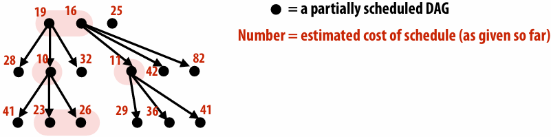
Challenge: might need to search over hundreds of thousands of possible schedules… how do we get the cost of a schedule?
Cost estimation using AI
Given program + schedule… estimate cost (in practice, doesn’t directly compute cost… it outputs 27 coefficients(系数) that are plugged into a hand-crafted cost model)
Simple MLP that runs in 10’s microseconds per schedule (e.g., 1.4M schedules tested in 166 seconds)
Trained on a large database of randomly generated Halide programs
Training programs compiled and executed to get actual cost
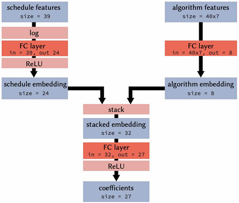
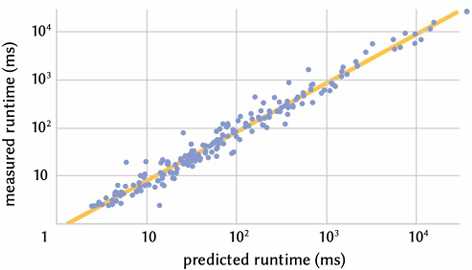
Autoscheduler comparable to best known human schedules
Graphs plot(绘制) relative throughput (output pixels/second)
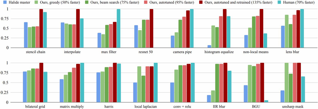
TL;DR - [Adams 2019], you’d have to work pretty hard to manually author a schedule that is better than the schedule generated by the Halide autoscheduler for image processing applications on CPUs
Autoscheduler saves time for experts
Earlier results from [Mullapudi 2016], not [Adams 2019]
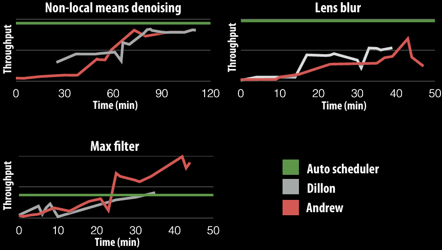
Takeaways(要点)
Halide scheduling primitives were designed to enhance productivity of expert human programmers that were trying to schedule image processing code
The high level of abstraction for scheduling also provided a clear way to enumerate the space of all possible schedules, enabling automated search
Consider searching over all possible permutations of a C++ program
Darkroom/Rigel/Aetherling
Goal: directly synthesize ASIC or FGPA implementation of image processing pipelines from a high-level algorithm description (a constrained “Halide-like” language)
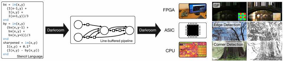
Goal: very-high e ciency image processing
Many other recent domain-speci c programming systems
hadoop
Less domain speci c than examples given today, but still designed specifically for: data-parallel computations on big data for distributed systems (“Map-Reduce”)
GraphLab
DSL for graph-based machine learning computations
Also see Ligra (DSLs for describing operations on graphs)
RAILS
Model-view-controller paradigm for web-applications
TensorFlow
DSL for de ning deep neural networks and training/inference computations on those networks
julia
Numerical computing
Ongoing e orts in many domains…
Languages for physical simulation: Simit [MIT], Ebb [Stanford]
Opt: a language for non-linear least squares optimization [Stanford]
Summary
Modern machines: parallel and heterogeneous
Only way to increase compute capability in energy-constrained world
Most software uses small fraction of peak capability of machine
Very challenging to tune programs to these machines
Tuning efforts are not portable across machines
Domain-specific programming environments trade-off generality to achieve productivity, performance, and portability
Case study today: Halide
Leverage explicit dependencies, domain restrictions, domain knowledge for system to synthesize efficient implementations
Another DSL example: Lizst: a language for solving PDE’s on meshes
[DeVito et al. Supercomputing 11, SciDac ’11]
What a Liszt program does
A Liszt program is run on a mesh(网格):
A Liszt program computes the value of fields defined on mesh faces, edges, or vertices
Liszt program: heat conduction(热传导) on mesh
Program computes the value of fields defined on meshes
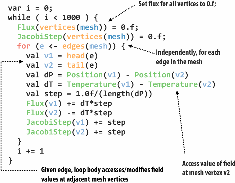
Liszt programming
A Liszt program describes operations on fields of an abstract mesh representation
Application specifies type of mesh (regular, irregular) and its topology(拓扑结构)
Mesh representation is chosen by Liszt (not by the programmer)
Based on mesh type, program behavior, and target machine
Well, that’s interesting. I write a program, and the compiler decides what data structure it should use based on what operations my code performs
Compiling to parallel computers
Recall challenges you have faced in your assignments
1.Identify parallelism
2.Identify data locality
3.Reason about what synchronization is required
Now consider how to automate this process in the Liszt compiler
Key: determining program dependencies
1.Identify parallelism
Absence of dependencies implies code can be executed in parallel
2.Identify data locality
Partition data based on dependencies
3.Reason about required synchronization
Synchronization is needed to respect dependencies (must wait until the values a computation depends on are known)
In general programs, compilers are unable to infer dependencies at global scale:
Consider: a[f(i)] += b[i];
(must execute f(i) to know if dependency exists across loop iterations i)
Liszt is constrained(受限) to allow dependency analysis
Lizst infers “stencils”: “stencil” = mesh elements accessed in an iteration of loop = dependencies for the iteration
Statically(静态) analyze code to find stencil of each top-level for loop
Extract(提取) nested mesh element reads
Extract operations on data at mesh elements
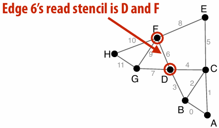
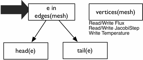
Portable(可移植) parallelism: compiler uses knowledge of dependencies to implement different parallel execution strategies
Strategy 1: mesh partitioning
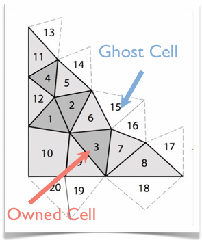
Strategy 2: mesh coloring
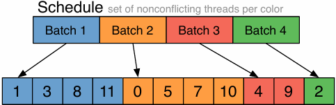
Imagine compiling a Lizst program to a cluster (multiple nodes, distributed address space) How might Liszt distribute a graph across these nodes?
Must access mesh elements relative to some input vertex, edge, face, etc.)
Notice how many operators return sets (e.g., “all edges of this face”)
Distributed memory implementation of Liszt
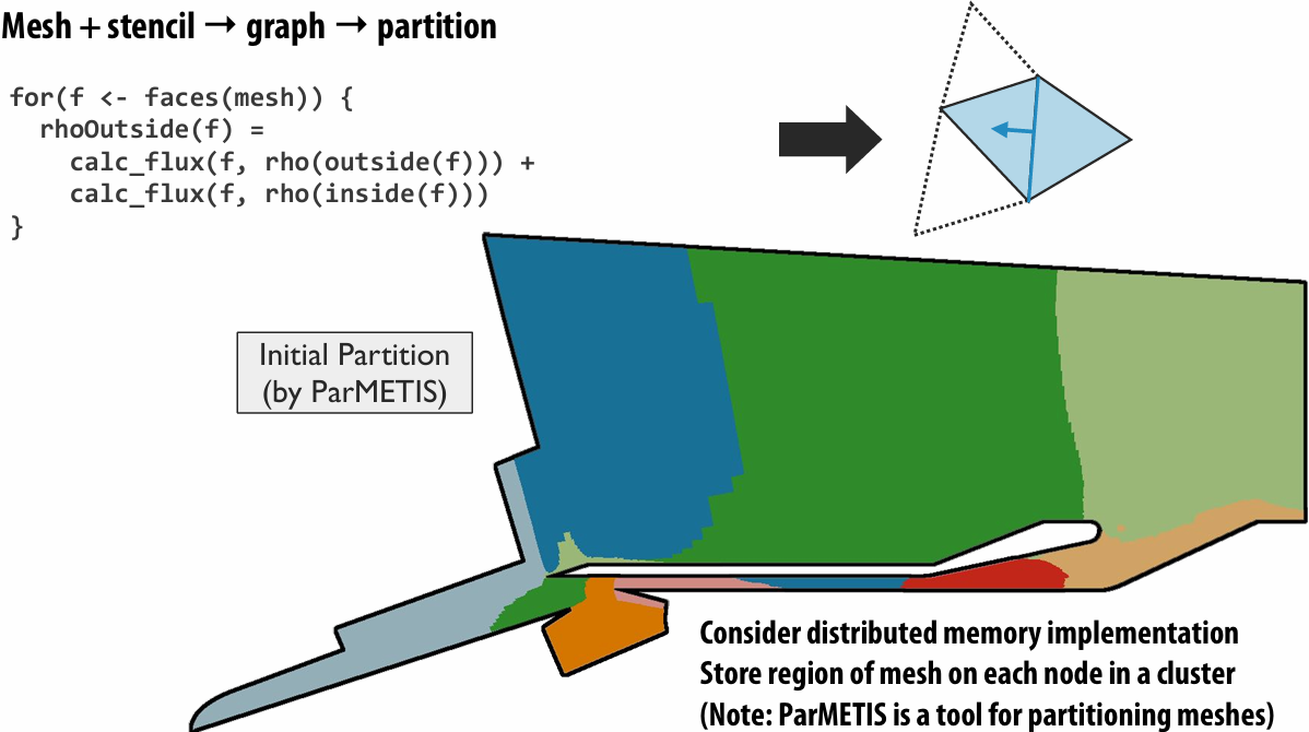
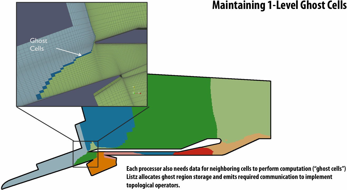
Imagine compiling a Lizst program to a GPU (single address space, many tiny threads)
GPU implementation: parallel reductions
In previous example, one region of mesh assigned per processor (or node in cluster)
On GPU, natural parallelization is one edge per CUDA thread
Edges (each edge assigned to 1 CUDA thread)
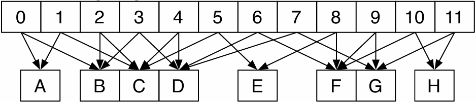
Flux field values (stored per vertex)
Different edges share a vertex: requires atomic update of per-vertex field data
GPU implementation: conflict graph
Edges (each edge assigned to 1 CUDA thread)
Flux field values (stored per vertex)
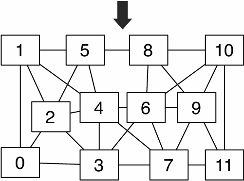
Identify mesh edges with colliding(冲突) writes (lines in graph indicate presence of collision)
Can simply run program once to get this information (results remain valid for subsequent executions provided mesh does not change)
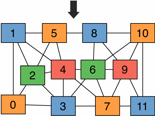
“Color” nodes in graph such that no connected nodes have the same color
Can execute on GPU in parallel, without atomic operations, by running all nodes with the same color in a single CUDA launch
Performance of Lizst program on a cluster
256 nodes, 8 cores per node (message-passing)
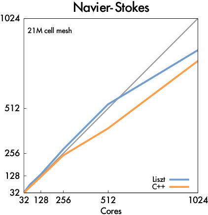
Important: performance portability!
Same Liszt program also runs with high efficiency on GPU (results not shown)
But uses a different algorithm when compiled to GPU! (graph coloring)
Liszt summary
Productivity
Abstract representation of mesh: vertices, edges, faces, fields (concepts that a scientist thinks about already!)
Intuitive topological(拓扑) operators
Portability
Same code runs on large cluster of CPUs and GPUs (and combinations thereof(其中)!)
High performance
Language is constrained to allow compiler to track dependencies
Used for locality-aware partitioning (distributed memory implementation)
Used for graph coloring to avoid sync (GPU implementation)
Compiler chooses different parallelization strategies for different platforms
System can customize mesh representation based on application and platform (e.g, don’t store edge pointers if code doesn’t need it)
Elements of good domain-speci c programming system design
#1: good systems identify the most important cases, and provide most bene t in these situations
Structure of code mimics(模仿) the natural structure of problems in the domain
Halide: pixel-wise view of filters: pixel(x,y) computed as expression of these input pixel values
Graph processing algorithms: per-vertex operations
Efficient expression: common operations are easy and intuitive to express
Efficient implementation: the most important optimizations in the domain are performed by the system for the programmer
My experience: a parallel programming system with “convenient” abstractions that precludes(排除) best-known implementation strategies will almost always fail
#2: good systems are simple systems
They have a small number of key primitives and operations
Halide: a few scheduling primitives for describing loop nests
Hadoop: map + reduce
Allows compiler/runtime to focus on optimizing these primitives
Provide parallel implementations, utilize appropriate hardware
Common question that good architects ask: “do we really need that?” (can this concept be reduced to a primitive we already have?)
For every domain-specific primitive in the system: there better be a strong performance or expressivity justification for its existence
#3: good primitives compose
Composition of primitives allows for wide application scope, even if scope is limited to a domain
e.g., frameworks discussed today support a wide variety of graph algorithms
Halide’s loop ordering + loop interleaving schedule primitives allow for expression of wide range of schedules
Composition often allows optimization to generalizable
If system can optimize A and optimize B, then it can optimize programs that combine A and B
Common sign that a feature should not be added (or added in a di erent way):
The new feature does not compose with all existing features in the system
Sign of a good design:
System ultimately is used for applications original designers never anticipated(预料)
LLM code generation
Trial and error via reflection
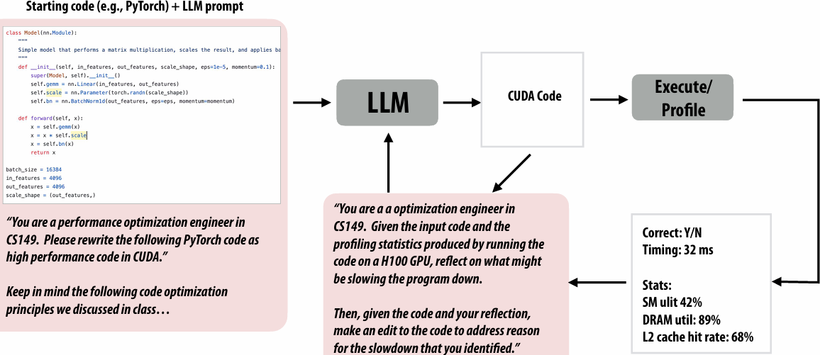
KernelBench
A benchmark of hundreds of PyTorch kernels
LMM agent’s goal is to automatically produce fast and correct CUDA kernels
https://github.com/ScalingIntelligence/KernelBench
Domain specific languages for writing DNN programs help automation as well
Good:
LLM is now assembling high-performance primitives, not writing low-level CUDA
Less likely for correctness mistakes/hallucinations(幻觉)
Challenge:
DNNs can struggle to write correct code in less-used languages (less data to train on… will resolve over time)
https://github.com/HazyResearch/ThunderKittens
https://triton-lang.org/main/index.html
https://github.com/NVIDIA/cutlass
https://github.com/tile-ai/tilelang
Open question: Can an LLM agent serve as a great CS149 student? At what token cost?
Idea 1: fine-tune LLMs based on experience
Use experience to fine-tune a custom LLM for a partial type of programming task
Need large numbers of tasks, ability to fine tune larger LLMs
Idea 2: LLM agent self-improves by building up a DB of “example solutions”
Agent builds up a database of example solutions (“e.g. practice problems”)
Given new problem to solve, it retrieves(检索) solutions to most relevant practice problems
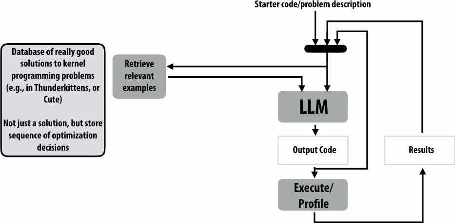
Benefit of database-driven self-improving agent
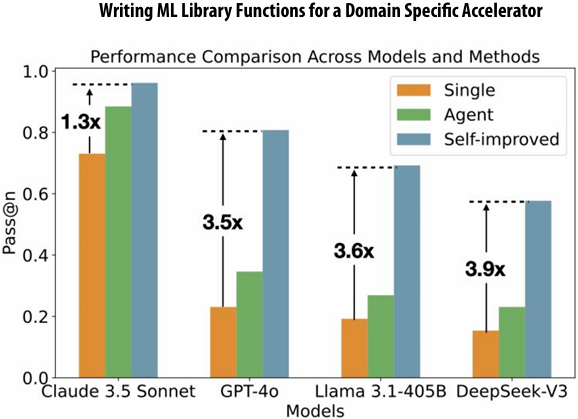
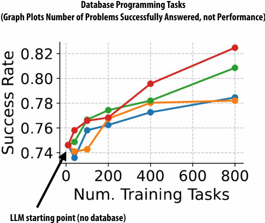
Idea 3: self-improvement via optimizing prompts from experience
Same idea as before, but now update the prompt given to the LLM based on the prior experience, don’t just provide relevant examples
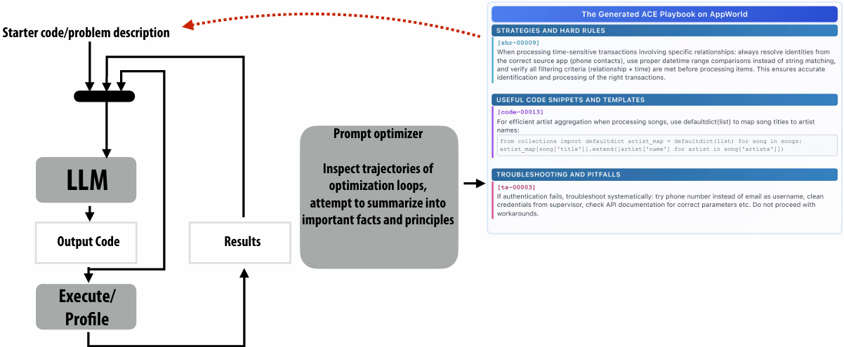
Idea 4:
Combine exhaustive(穷举) search based techniques (like the Halide autotune), with the LLM agentic ideas above
Extremely high optimization cost, but some of the best results
<style>.fqkvmzzkklej{zoom:80%;}</style>{% asset_img fqkvmzzkklej image-20260210000311334.png '"""image-20260210000311334"' %}
Summary
Performance optimization requires a high level of expertise
And even for experts it’s tedious and hard
And have to repeat it for new machines, slightly different problems
And companies are spending 10’s to 100’s of millions of dollars a year or more on AI compute costs
Seems like a great case for automation
The best cs149 students of the future will likely be able to work in tangent with(协同) automatic agents to accelerate their thinking and their work
Interesting debates on whether the real value that leads to success is in the DSL design, or the LLM agent!!!!
Lecture 14: Cache Coherence
Cache Design
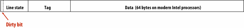
the difference between a write back and a write-through cache
write through says when we do the write to the cache, we also write to the main memory, and write back says we only write to the cache, and later the data is actually written to main memory
a write-allocate vs. write-no-allocate cache
So the question is, what happens when I write to the cache, and the line that I want is not there? Do I allocate? Do I actually fetch the rest of the line and write into the cache? Or do I just write directly to main memory?
Behavior of write-allocate, write-back cache on a write miss (uniprocessor case)
Example: processor executes int x = 1;
1.Processor performs write to address that “misses” in cache
2.Cache selects location to place line in cache, if there is a dirty line currently in this location, the dirty line is written out to memory
3.Cache loads line from memory (“allocates line in cache”)
4.Whole cache line is fetched and 32 bits are updated
5.Cache line is marked as dirty
Cache hierarchy of Intel Skylake CPU (2015)
Caches exploit locality
64 byte cache line size
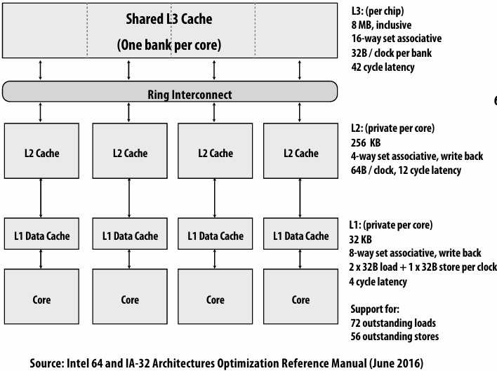
3 Cs cache miss model
Cold
Capacity
Conflict
A shared memory multi-processor
Processors read and write to shared variables
More precisely: processors issue load and store instructions
A reasonable expectation of memory is:
Reading a value at address X should return the last value written to address X by any processor
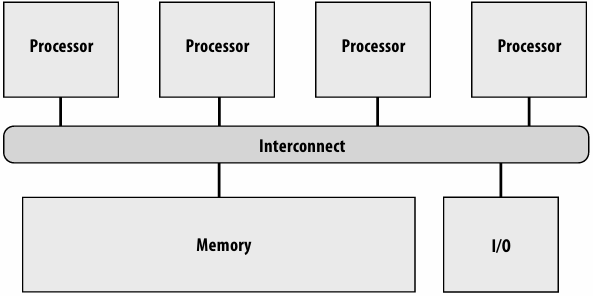
(A simple view of four processors and their shared address space)
Cache coherence problem
Modern processors replicate contents of memory in local caches
Problem: processors can observe different values for the same memory location
This is a problem created by replicating the data in local caches, can not fix the problem by adding locks to program
Intuitive expectation of shared memory
Intuitive behavior for memory system: reading value at address X should return the last value written to address X by any processor
Memory coherence problem exists because there is both global storage (main memory) and per-processor local storage (processor caches) implementing the abstraction of a single shared address space
On a uniprocessor(单处理器), providing this behavior is fairly simple, since writes typically come from one source: the processor
Exception: device I/O via direct memory access (DMA)
Problems with the intuition
Intuitive behavior: reading value at address X should return the last value written to address X by any processor
What does “last” mean?
What if two processors write at the same time?
What if a write by P1 is followed by a read from P2 so close in time that it is impossible to communicate the occurrence of the write to P2 in time?
In a sequential program, “last” is determined by program order (not time)
Holds true within one thread of a parallel program
But we need to come up witha meaningful way to describe order across threads in a parallel program
Coherence
Definition: Coherence
A memory system is coherent if:
The results of a parallel program’s execution are such that for each memory location , there is a hypothetical(假想的) serial order of all program operations (executed by all processors) to the location that is consistent with the results of execution, and:
1.Memory operations issued by any one processor occur in the order issued by the processor
2.The value returned by a read is the value written by the last write to the location… as given by the serial order
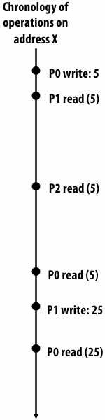
Implementation: Cache Coherence Invariants(不变量)
For any memory address x, at any given time period (epoch):
Single-Writer, Multiple-Read (SWMR) Invariant
Read-write epoch: there exists only a single processor that may write to x (and can also read it)
Read-Only- epoch: some number of processors that may only read x
Data-Value Invariant (write serialization)
The value of the memory address at the start of an epoch is the same as the value of the memory location at the end of its last read-write epoch

Implementing coherence
Software-based solutions (coarse grain: VM page)
OS uses page-fault(缺页) mechanism to propagate(传播) writes
Can be used to implement memory coherence over clusters of workstations
We won’t discuss these solutions
Big performance problem: false sharing
Hardware-based solutions (fine grain: cache line)
“Snooping(窥探)”-based coherence implementations
Directory(目录)-based coherence implementations
Shared caches: coherence made easy
One single cache shared by all processors
Eliminates problem of replicating state in multiple caches
Obvious scalability problems (since the point of a cache is to be local and fast)
Interference(干扰) (conflict misses) / contention(争用) due to many clients (destructive)
But shared caches can have benefits:
Facilitates(便于) fine-grained sharing (overlapping working sets)
Loads/stores by one processor might pre-fetch lines for another processor (constructive)
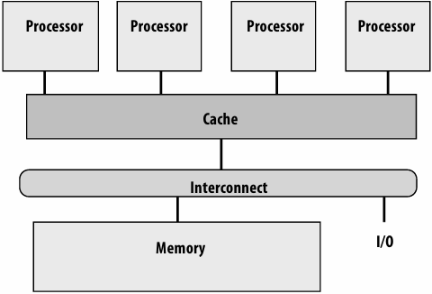
“Snooping”-based coherence implementations
Snooping cache-coherence schemes
Main idea: all coherence-related activity is broadcast to all processors in the system (more specifically: to the processor’s cache controllers)
Cache controllers monitor (“they snoop”) memory operations, and follow cache coherence protocol to maintain memory coherence
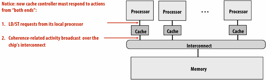
Very simple coherence implementation
Let’s assume:
1.Write-through caches
2.Granularity of coherence is cache line
Coherence Protocol:
Upon write, cache controller broadcasts invalidation message
As a result, the next read from other processors will trigger cache miss
(processor retrieves updated value from memory due to write-through policy)
$ mean cache
| Action | Interconnect activity | P0 $ | P1 $ | mem location X |
|---|---|---|---|---|
| 0 | ||||
| P0 load X | cache miss for X | 0 | 0 | |
| P1 load X | cache miss for X | 0 | 0 | 0 |
| P0 write 100 to X | invalidation for X | 100 | 100 | |
| P1 load X | cache miss for X | 100 | 100 | 100 |
Write-through policy is inefficient
Every write operation goes out to memory
Very high bandwidth requirements
Write-back caches absorb most write traffic as cache hits
Significantly reduces bandwidth requirements
But now how do we maintain cache coherence invariants?
This requires more sophisticated coherence protocols
Cache coherence with write-back caches
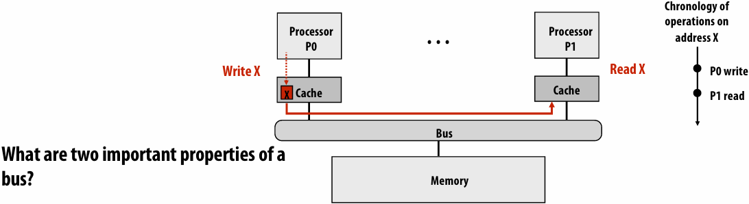
broadcast and serialization
Dirty state of cache line now indicates exclusive ownership (Read-Write Epoch)
Modified: cache is only cache with a valid copy of line (it can safely be written to)
Owner: cache is responsible for propagating information to other processors when they attempt to load it from memory (otherwise a load from another processor will get stale(旧的) data from memory)
Cache Coherence Protocol
Algorithm that maintains cache coherent invariants
The logic we are about to describe is performed by each processor’s cache controller in response to:
Loads and stores by the local processor
Messages from other caches on the bus
If all cache controllers operate according to this described protocol, then coherence will be maintained
The caches “cooperate” to ensure coherence is maintained
Invalidation-based write-back protocol
Key ideas:
A line in the “modified” state can be modified without notifying the other caches
Processor can only write to lines in the modified state
Need a way to tell other caches that processor wants exclusive access to the line
We accomplish this by sending message to all the other caches
When cache controller sees a request for modified access to a line it contains
It must invalidate the line in its cache
cache line state bits
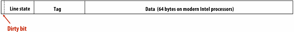
MSI write-back invalidation protocol
Key tasks of protocol
Ensuring processor obtains exclusive access for a write
Locating most recent copy of cache line’s data on cache miss
Three cache line states
Invalid (I): same as meaning of invalid in uniprocessor cache
Shared (S): line valid in one or more caches, memory is up to date
Modified (M): line valid in exactly one cache (a.k.a. “dirty” or “exclusive” state)
Two processor operations (triggered by local CPU)
PrRd(read)
PrWr(write)
Three coherence-related bus transactions (from remote caches)
BusRd: obtain copy of line with no intent to modify
BusRdX: obtain copy of line with intent to modify
BusWB: write dirty line out to memory
Cache Coherence Protocol: MSI State Transition Diagram
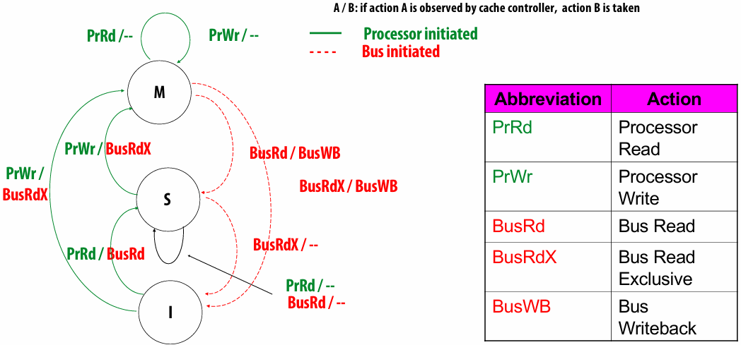
MSI Invalidate Protocol
Read obtains block in “shared”
even if only cached copy
Obtain exclusive ownership before writing
BusRdX causes others to invalidate
If M in another cache, will cause writeback
BusRdX even if hit in S
promote to M (upgrade)
all caches are carrying out this logic independently to maintain coherence
A Cache Coherence Example
| Proc Action | P1 $-state | P2 $-state | P3 $-state | Bus Trans | Data from |
|---|---|---|---|---|---|
| P1 read x | S | -- | -- | BusRd | Memory |
| P3 read x | S | -- | S | BusRd | Memory |
| P3 write x | I | -- | M | BusRdX | Memory |
| P1 read x | S | -- | S | BusRd | P3 $ |
| P1 read x | S | -- | S | P1 $ | |
| P2 write x | I | M | I | BusRdX | Memory |
Single writer, multiple reader protocol
Why do you need Modified to Shared?
the invariant we’re trying to maintain is single-writer, multiple-reader. So in order to track that transition, we need the transition from modified to share
Communication increases memory latency
How Does MSI Satisfy Cache Coherence?
1.Single-Writer, Multiple-Read (SWMR) Invariant
2.Data-Value Invariant (write serialization)
Summary: MSI
A line in the M state can be modified without notifying other caches
No other caches have the line resident, so other processors cannot read these values (without generating a memory read transaction)
Processor can only write to lines in the M state
If processor performs a write to a line that is not exclusive in cache, cache controller must first broadcast a transaction to move the line into that state
Read-exclusive tells other caches about impending(即将) write (“you can’t read any more, because I’m going to write”)
Read-exclusive transaction is required even if line is valid (but not exclusive… it’s in the S state) in processor’s local cache
Dirty state implies exclusive
When cache controller snoops a “read exclusive” for a line it contains
Must invalidate the line in its cache
Because if it didn’t, then multiple caches will have the line (and soit wouldn’t be exclusive in the other cache!)
MESI invalidation protocol
MSI requires two interconnect transactions for the common case of reading an address, then writing to it
Transaction 1: BusRdto move from I to S state
Transaction 2: BusRdXto move from S to M state
This inefficiency exists even if application has no sharing at all
Solution: add additional state E (“exclusive clean”)
Line has not been modified, but only this cache has a copy of the line
Decouples(解耦) exclusivity from line ownership (line not dirty, so copy in memory is valid copy of data)
Upgrade from E to M does not require anbustransaction
MESI state transition diagram
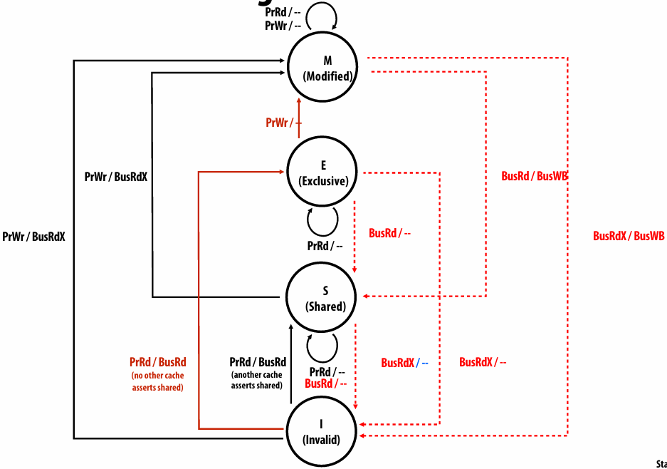
So you go from invalid to shared would be the typical case, if the line was shared
But if the line were not shared, then you could go directly to exclusive state
And now the upgrade can be made without doing a bus transaction
example:
if you did a write first, I want to read first and then write
Directory-based coherence implementations
Scalable cache coherence using directories
Snooping schemes broadcast coherence messages to determine the state of a line in the other caches: not scalable
Alternative idea: avoid broadcast by storing information about the status of the line in one place: a “directory”
The directory entry for a cache line contains information about the state of the cache line in all caches
Caches look up information from the directory as necessary
Cache coherence is maintained by point-to-point messages between the caches on a “need to know” basis (not by broadcast mechanisms)
Directory instead of bus serves as coherence serialization mechanism
Still need to maintain invariants
SWMR
Write serialization
Directory coherence in Intel Core i7 CPU
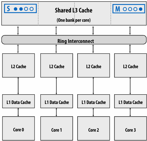
L3 serves as centralized(集中式) directory for all lines in the L3 cache
Serialization piont
(Since L3 is an inclusive cache, any line in L2 is guaranteed to also be resident in L3)
Directory maintains list of L2 caches containing line
Instead of broadcasting coherence traffic to all L2’s, only send coherence messages to L2’s that contain the line
(Core i7 interconnect is a ring, it is not a bus)
Directory dimensions:
P=4
M = number of L3 cache lines
Implications of cache coherence to the programmer
Communication Overhead
Communication time is a key parallel overhead
Appears as increased memory access time in multiprocessor
Extra main memory accesses in UMA systems(均匀访存模型(Uniform Memory Access,UMA)是一种并行体系结构中的内存访存模型,其特点是所有处理器访问内存的时间相同,亦称统一内存存取或紧耦合系统)
Must determine increase in cache miss rate vs. uniprocessor
Some accesses have higher latency in NUMA systems(非统一内存访问(NUMA)是一种用于多处理器的电脑内存体设计,内存访问时间取决于处理器的内存位置。 在NUMA下,处理器访问它自己的本地存储器的速度比非本地存储器(存储器的地方到另一个处理器之间共享的处理器或存储器)快一些)
Only a fraction of a % of these can be significant!
AMATMultiprocessor > AMATUniprocessor
Use system tools to optimize cache performance
Intel VTune
Get Intel® VTune™ Profiler
Apple Xcode Instruments
Instruments Tutorials | Apple Developer Documentation
Unintended communication via false sharing
What is the potential performance problem with this code?
有多个数据在同一个 cache line,写数据时需要频繁执行切换写回,conflict
1 | // allocate per-thread variable for local per-thread accumulation |
Why might this code be more performant?
数据分散在不同 cache line,写数据时不需要频繁执行切换写回,conflict
1 | // allocate per thread variable for local accumulation |
Demo: false sharing
threads update a per-thread counter many times
1 | void* worker(void* arg) { |
Execution time with num_threads=8 on 4-core system: 14.2 sec
1 | void test1(int num_threads) { |
Execution time with num_threads=8 on 4-core system: 4.7 sec
1 | struct padded_t { |
False sharing
Condition where two processors write to different addresses, but addresses map to the same cache line
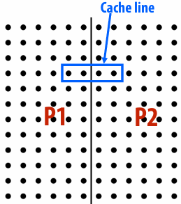
Cache line “ping-pongs” between caches of writing processors, generating significant amounts of communication due to the coherence protocol
No inherent communication, this is entirely artifactual communication (cachelines > 4B)
False sharing can be a factor in when programming for cache coherent architectures
Impact of cache line size on miss rate
Results from simulation of a 1 MB cache (four example applications)
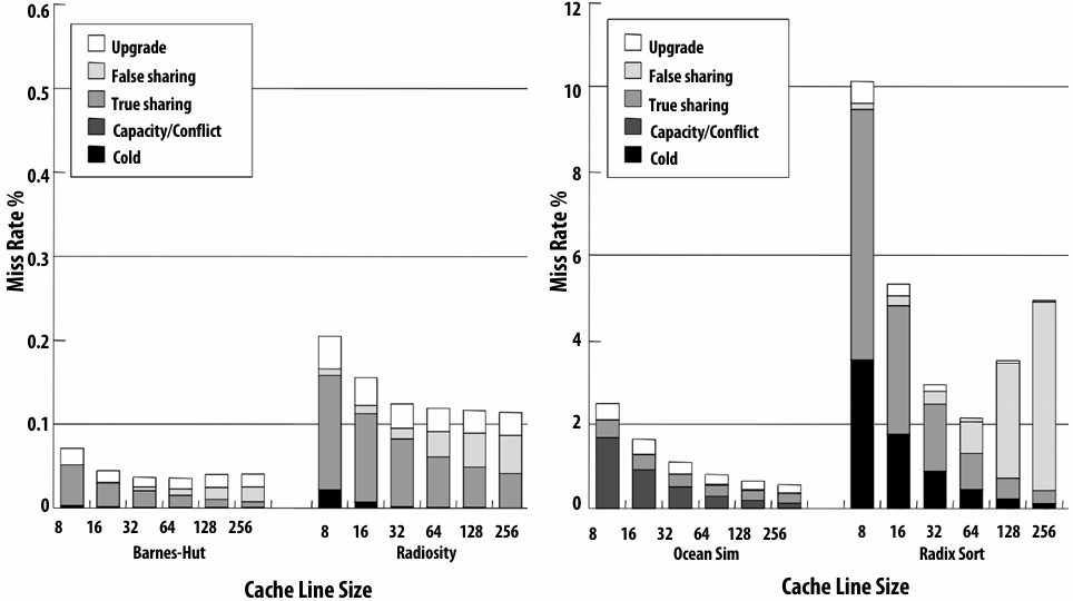
Note: I separated the results into two graphs because of different Y-axis scales
Summary: Cachecoherence
The cache coherence problem exists because the abstraction of a single shared address space is not implemented by a single storage unit
Storage is distributed among main memory and local processor caches
Data is replicated in local caches for performance
Main idea of snooping-based cache coherence: whenever a cache operation occurs that could affect coherence, the cache controller broadcasts a notification to all other cache controllers in the system
Challenge for HW architects: minimizing overhead of coherence implementation
Challenge for SW developers: be wary of artifactual communication due to coherence protocol (e.g., false sharing)
Scalability of snooping implementations is limited by ability to broadcast coherence messages to all caches!
Scaling cache coherence via directory-based approaches
Lecture 15: Memory Coherency and Consistency
Shared Memory Behavior
Intuition says loads should return latest value written
What is latest?
Coherence: only one memory address
Consistency: apparent ordering for all addresses
Order in which memory operations performed by one thread become visible to other threads
Affects
Programmability: how programmers reason about program behavior
Allowed behavior of multithreaded programs executing with shared memory
Performance: limits HW/SW optimizations that can be used
Reordering memory operations to hide latency
Memory Consistency: Who Should Care
Anyone who:
Wants to implement a synchronization library
Will ever work a job in kernel (or driver) development
Seeks to implement lock-free data structures
Memory coherence vs. memory consistency
Memory coherence defines requirements for the observed behavior of reads and writes to the same memory location
All processors must agree on the order of reads/writes to X
In other words: it is possible to put all operations involving X on a timeline such that the observations of all processors are consistent with that timeline
Memory consistency defines the behavior of reads and writes to different locations (as observed by other processors)
Coherence only guarantees that writes to address X will eventually propagate to other processors
Consistency deals with when writes to X propagate to other processors, relative to reads and writes to other addresses
Coherence vs. Consistency (said again, perhaps more intuitively this time)
The goal of cache coherence is to ensure that the memory system in a parallel computer behaves as if the caches were not there
Just like how the memory system in a uni-processor system behaves as if the cache was not there
A system without caches would have no need for cache coherence
Memory consistency defines the allowed behavior of loads and stores to different addresses in a parallel system
The allowed behavior of memory should be specified whether or notcaches are present (and that’s what a memory consistency model does)
Memory Consistency
TL:DR:(简而言之)
Multiprocessors reorder memory operations in unintuitive and strange ways
This behavior is necessary for performance
Application programmers rarely see this behavior
Systems (OS and compiler) developers see it all the time
Memory operation ordering
A program defines a sequence of loads and stores (this is the “program order” of the loads and stores)
Four types of memory operation orderings
WX→RY: write to X must commit before subsequent read from Y
RX →RY: read from X must commit before subsequent read from Y
RX →WY: read to X must commit before subsequent write to Y
WX →WY: write to X must commit before subsequent write to Y
To clarify: “write must commit before subsequent read” means:
When a write comes before a read in program order, the write must commit (its results are visible) by the time the read occurs
Example: Multiprocessor Execution
Initially A = B = 0Proc 0 Proc 1(1) A = 1 (3) B = 1(2) print B (4) print A
What can be printed?
“01”?
“10”?
“11”?
“00”?
Orderings That Should Not Happen
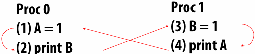
The program should not print “00” or “10”
A “happens-before” graph shows the order in which events must execute to get a desired outcome
If there’s a cycle in the graph, an outcome is impossible—an event must happen before itself!
Sequential consistency
What Should Programmers Expect
Sequential Consistency
Lamport 1976 (Turing Award 2013)
All operations executed in some sequential order
As if they were manipulating a single shared memory
Each thread’s operations happen in program order
A sequentially consistent memory system maintains all four memory operation orderings (WX →RY, RX→RY, RX→WY, WX→WY)
There is a chronology of all memory operations that is consistent with observed values
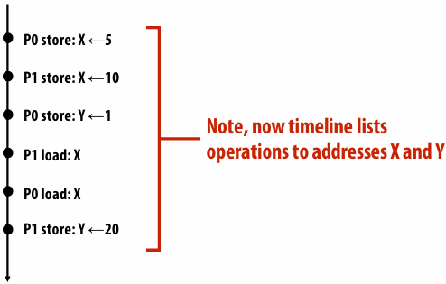
Sequential consistency (switch metaphor)
All processors issue loads and stores in program order
Memory chooses a processor at random, performs a memory operation to completion, then chooses another processor, …
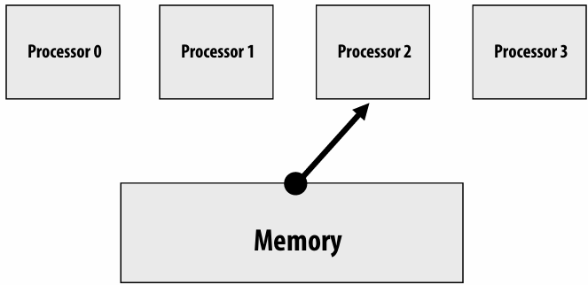
Sequential Consistency Example
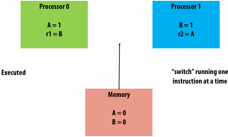
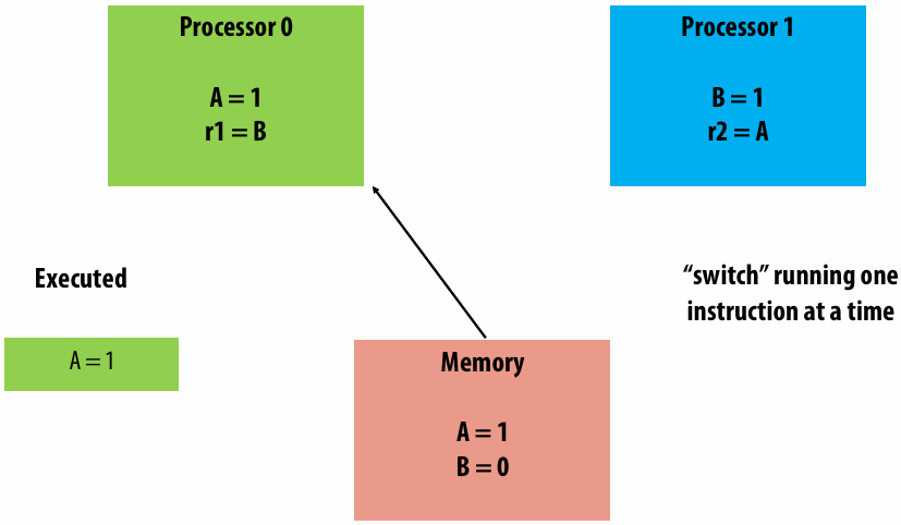
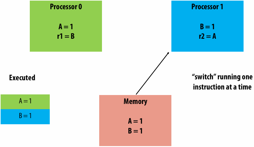
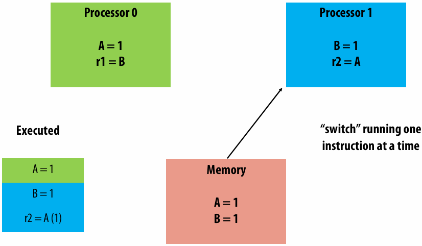
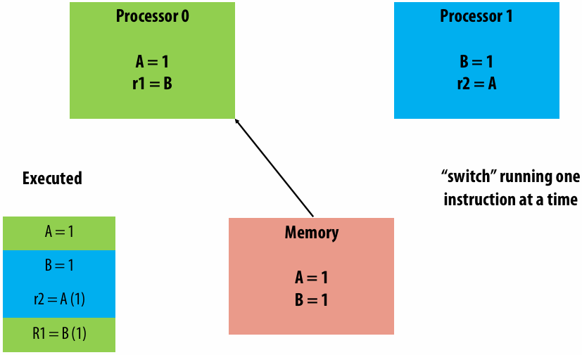
Relaxing memory operation ordering
A sequentially consistent memory system maintains all four memory operation orderings (WX →RY, RX→RY, RX→WY, WX→WY)
Relaxed memory consistency models allow certain orderings to be violated(违反)
Motivation for relaxed consistency: hiding latency
Why are we interested in relaxing ordering requirements?
To gain performance
Specifically, hiding memory latency: overlap memory access operations with other operations when they are independent
Remember, memory access in a cache coherent system may entail(包含) much more work then simply reading datafrom memory (finding data, sending invalidations, etc.)
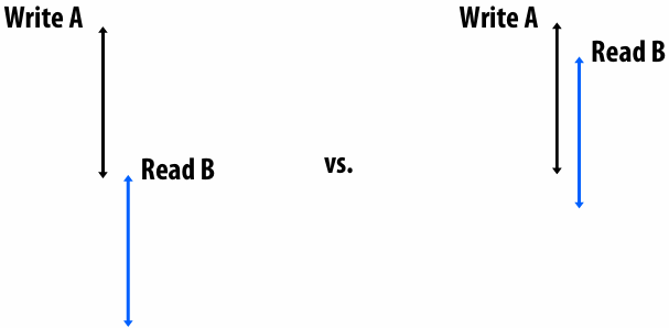
Problem with SC
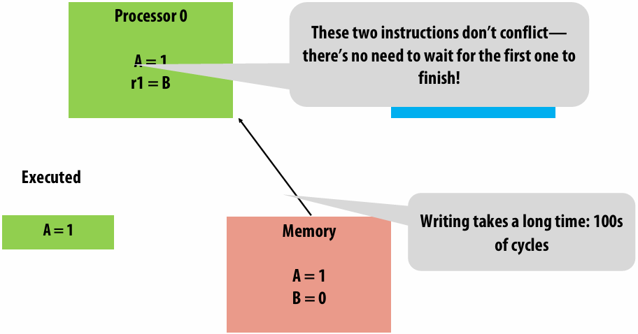
Optimization: Write Buffer
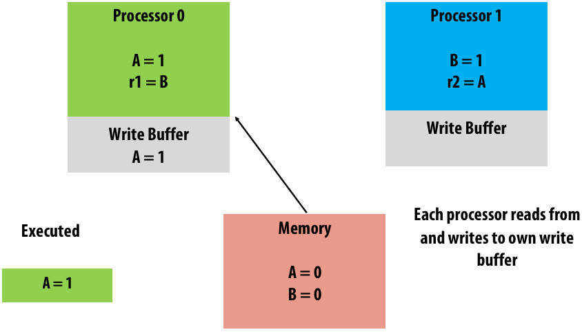
Initially A = B = 0
Proc 0 Proc 1
(1) A = 1 (3) B = 1
(2) r1 = B (4) r2 = A
Can r1 = r2 = 0?
SC: No
Write buffers: Yes
Write Buffer Performance
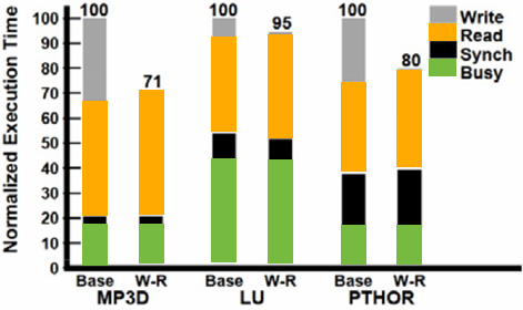
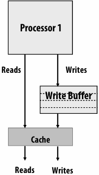
Base: Sequentially consistent execution. Processor issues one memory operation at a time, stalls until completion
W-R: relaxed W→R ordering constraint (write latency almost fully hidden)
Write Buffers: Who Cares?
Performance improvement
Every modern processor uses them
Intel x86, ARM, RISC-V
Need a weaker memory model
TSO: Total Store Order
Slightly harder to reason about than SC
x86 uses an incompletely specified form of TSO
Allowing reads to move ahead of writes
Four types of memory operation orderings
WX → RY: write must complete before subsequent read
RX → RY: read must complete before subsequent read
RX → WY: read must complete before subsequent write
WX → WY: write must complete before subsequent write
Allow processor to hide latency of writes
Total Store Ordering (TSO)
Processor Consistency (PC)
Total store ordering (TSO)
Processor P can read B before its write to A is seen by all processors (processor can move its own reads in front of its own writes)
Reads by other processors cannot return new value of A until the write to A is observed by all processors
Processor consistency (PC)
Any processor can read new value of A before the write is observed by all processors
In TSO and PC, only WX → RY order is relaxed. The WX → WY constraint still exists. Writes by the same thread are not reordered (they occur in program order)
Clarification (make sure you get this!)
The cache coherency problem exists because hardware implements the optimization of duplicating data in multiple processor caches. The copies of the data must be kept coherent
Relaxed memory consistency issues arise from the optimization of reordering memory operations. (Consistency is unrelated to whether or notcaches exist in the system)
Allowing writes to be reordered
Four types of memory operation orderings
WX→RY: write complete before subsequent read
RX →RY: read must complete before subsequent read
RX →WY: read must complete before subsequent write
WX →WY: write must complete before subsequent write
Partial Store Ordering (PSO)
Execution may not match sequentialconsistency on program 1 (P2 may observe change to flag before change to A)
Thread 1 (on P1) Thread 2 (on P2)
A = 1; while (flag == 0);
flag = 1; print A;
**Why might it be useful to allow more aggressive(激进的) memory operation reorderings? **
WX → WY: processor might reorder write operations in a write buffer (e.g., one is a cache miss while the other is a hit)
RX → WY, RX → RY: processor might reorder independent instructions in an instruction stream (out-of-order execution)
Keep in mind these are all valid optimizations if a program consists of a single instruction stream
Allowing all reorderings
Four types of memory operation orderings
WX→RY: write complete before subsequent read
RX →RY: read must complete before subsequent read
RX →WY: read must complete before subsequent write
WX →WY: write must complete before subsequent write
No guarantees about operations on data!
Everything can be reordered
Motivation is increased performance
Overlap multiple reads and writes in the memory system
Execute reads as early as possible and writes as late as possible to hide memory latency
Examples:
Weak ordering (WO)
Release Consistency (RC)
Synchronization
Synchronization to the Rescue
Memory reordering seems like a nightmare (it is!)
Every architecture provides synchronization primitives to make memory ordering stricter
Fence (memory barrier) instructions prevent reorderings, but are expensive
All memory operations complete before any memory operation after it can begin
reorderable reads and writes here
...
MEMORY FENCE
...
reorderable reads and writes here
...
MEMORY FENCE
Other synchronization primitives (per address):
read-modify-write/compare-and-swap, transactional memory, …
Example: expressing synchronization in relaxed models
Intel x86/x64 ~ total store ordering
Provides sync instructions if software requires a specific instruction ordering not guaranteed by the consistency model
mm_lfence (“load fence”: wait for all loads to complete)
mm_sfence (“store fence”: wait for all stores to complete)
mm_mfence (“mem fence”: wait for all me operations to complete)
ARM processors: very relaxed consistency model
A cool post on the role of memory fences in x86:
http://bartoszmilewski.com/2008/11/05/who-ordered-memory-fences-on-an-x86/
ARM has some great examples in their programmer’s reference:
http://infocenter.arm.com/help/topic/com.arm.doc.genc007826/Barrier_Litmus_Tests_and_Cookbook_A08.pdf
A great list of academic papers:
http://www.cl.cam.ac.uk/~pes20/weakmemory/
Problem: Data Races
Every example so far has involved a data race
Two accesses to the same memory location
At least one is a write
Unordered by synchronization operations
Conflicting data accesses
Two memory accesses by different processors conflict if…
They access the same memory location
At least one is a write
Unsynchronized program
Conflicting accesses not ordered by synchronization (e.g., a fence, operation with release/acquire semantics, barrier, etc.)
Unsynchronized programs contain data races: the output of the program depends on relative speed of processors (non-deterministic program results)
Synchronized Programs
Synchronized programs yield SC results on non-SC systems
Synchronized programs are data-race-free
If there are no data races, reordering behavior doesn’t matter
Accesses are ordered by synchronization, and synchronization forces sequential consistency
In practice, most programs you encounter will be synchronized (via locks, barriers, etc. implemented in synchronization libraries)
Rather than via ad-hoc reads/writes to shared variables like in the example programs
Summary: Relaxed Consistency
Motivation: obtain higher performance by allowing reordering of memory operations (reordering is not allowed by sequential consistency)
One cost is software complexity: programmer or compiler must correctly insert synchronization to ensure certain specific operation orderings when needed
But in practice complexities encapsulated in libraries that provide intuitive primitives like lock/unlock, barrier (or lower-level primitives like fence)
Optimize for the common case: most memory accesses are not conflicting, so don’t design a system that pays the cost as if they are
Relaxed consistency models differ in which memory ordering constraints they ignore
Language Level Memory Models
Languages Need Memory Models Too
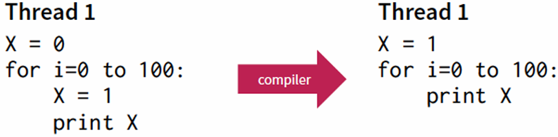
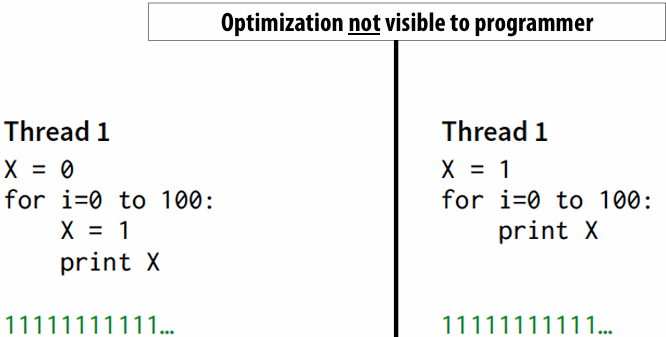
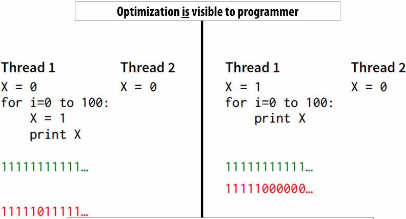
Provide a contract to programmers about how their memory operations will be reordered by the compiler e.g. no reordering of shared memory operations
Modern (C11, C++11) and not-so-modern (Java 5) languages guarantee sequential consistency for data-race-free programs (“SC for DRF”)
Compilers will insert the necessary synchronization to cope with the hardware memory model
No guarantees if your program contains data races!
The intuition is that most programmers would consider a racy program to be buggy
Use a synchronization library!
Memory Consistency Models Summary
Define the allowed reorderings of memory operations by hardware and compilers
A contract between hardware or compiler and application software
Weak models required for good performance?
SC can perform well with many more resources
Details of memory model can be hidden in synchronization library
Requires data race free (DRF) programs
Lecture 16: Implementing Locks, Fine-Grained Synchronization, and (a short intro to) Lock-Free Programming
Deadlock Livelock Starvation
(Deadlock and livelock concern program correctness. Starvation is really an issue of fairness.)
Deadlock
Deadlock is a state where a system has outstanding(未完成的) operations to complete, but no operation can make progress
Deadlock can arise when each operation has acquired a shared resource that another operation needs
In a deadlock situations, there is no way for any thread to make progress unless some thread relinquishes a resource
Required conditions for deadlock
Mutual exclusion: only one processor can hold a given resource at once
Hold and wait: processor must hold the resource while waiting for other resources it needs to complete an operation
No preemption: processors don’t give up resources until operation they wish to perform is complete
Circular wait: waiting processors have mutual dependencies (a cycle exists in the resource dependency graph)
Livelock
Livelock is a state where a system is executing many operations, but no thread is making meaningful progress
Starvation
State where a system is making overall progress, but some processes make no progress
Starvation is usually not a permanent(永久的) state
Lock implementations
Test-and-set based lock
Atomic test-and-set instruction:
ts R0, mem[addr] // load mem[addr] into R0
// if mem[addr] is 0, set mem[addr] to 1
lock: ts R0, mem[addr] // load word into R0
bnz R0, lock // if 0, lock obtained
unlock: st mem[addr], #0 // store 0 to address
x86 cmpxchg
Compare and exchange (atomic when used with lock prefix)
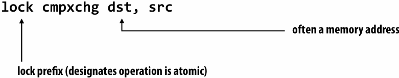
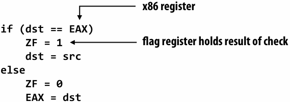
Test-and-set lock: consider coherence traffic
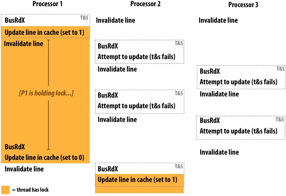
what is the duration of time the thread running on P1 holds the lock?
It was the entire time
At what points in time does P1’s cache contain a valid copy of the cache line containing the lock variable?
Was only for a second at the time of lock, and for a split second at the time of unlock
Test-and-set lock performance
Benchmark: execute a total of N lock/unlock sequences (in aggregate) by P processors
Critical section time removed so graph plots only time acquiring/releasing the lock
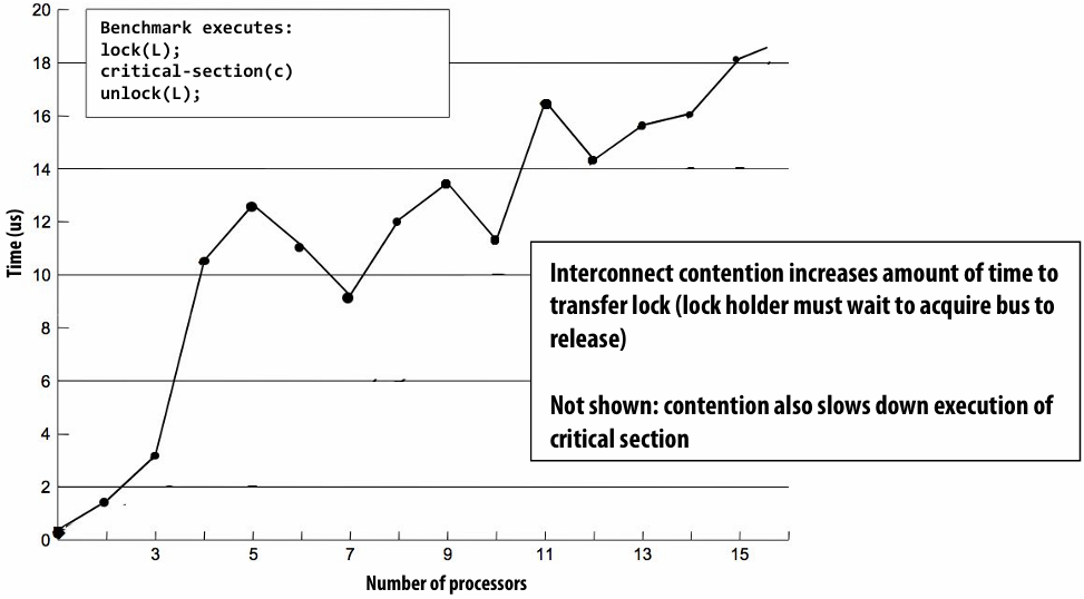
Desirable lock performance characteristics
Low latency
If lock is free and no other processors are trying to acquire it, a processor should be able to acquire the lock quickly
Low interconnect traffic
If all processors are trying to acquire lock at once, they should acquire the lock in succession(依次) with as little traffic as possible
Scalability
Latency / traffic should scale reasonably with number of processors
Low storage cost
Fairness
Avoid starvation or substantial unfairness
One ideal: processors should acquire lock in the order they request access to it
Simple test-and-set lock: low latency (under low contention), high traffic, poor scaling, low storage cost (one int), no provisions for fairness
Test-and-test-and-set lock
1 | void Lock(int* lock) { |
Test-and-test-and-set lock: coherence traffic
Test-and-test-and-set characteristics
Slightly higher latency than test-and-set in no contention case
Must test… then test-and-set
Generates much less interconnect traffic
One invalidation, per waiting processor, per lock release (O(P) invalidations)
This is O(P2) interconnect traffic if all processors have the lock cached
Recall: test-and-set lock generated one invalidation per waiting processor per test
More scalable (due to less traffic)
Storage cost unchanged (one int)
Still no provisions for fairness
Another impl: ticket lock
Main problem with test-and-set style locks: upon release, all waiting processors attempt to acquire lock using test-and-set
1 | struct lock { |
No atomic operation needed to acquire the lock (only a read)
Result: only one invalidation per lock release (O(P) interconnect traffic)
Atomic operations (provided by CUDA)
1 | int atomicAdd(int* address, int val); |
(omitting(省略) additional 64 bit and unsigned int versions)
Implementing atomic fetch-and-op
Example: atomic_min()
1 | // atomicCAS: (“compare and swap”) |
1 | void atomic_min(int* addr, int x) { |
Exercise: how can you build an atomic fetch+op out of atomicCAS()?
1 | // for signed values of x |
Another exercise: build a lock
1 | typedef int lock; |
Load-linked, store conditional (LL/SC)
Pair of corresponding instructions (not a single atomic instruction like compare-and swap)
load_linked(x): load value from address
store_conditional(x, value): store value to x, if x hasn’t been written to by any processor since the corresponding load linked operation
Corresponding ARM instructions: LDREX and STREX
How might LL/SC be implemented on a cache coherent processor?
LL/SC 的实现依赖于每核一个的链接状态寄存器。load_linked 记录地址并设置标志;利用 MESI 协议的作废机制,当地址被其他核心修改时,通过监听总线自动清空标志;store_conditional 只需检查标志位即可确定数据是否在此期间被动过
C++ 11 atomic<T>
Provides atomic read, write, read-modify-write of entire objects
Atomicity may be implemented by mutex or efficiently by processor-supported atomic instructions (if T is a basic type)
Provides memory ordering semantics for operations before and after atomic operations
By default: sequential consistency
See std::memory_order or more detail
1 | atomic<int> i; |
Using locks: Fine-grained locking examples
Example: a sorted linked list
What can go wrong if multiple threads operate on the linked list simultaneously?
1 | struct Node { |
Example: simultaneous insertion
Thread 1 attempts to insert 6
Thread 2 attempts to insert 7
Thread 1 and thread 2 both compute same prev and cur
Result: one of the insertions gets lost!
Result: (assuming thread 1 updates prev->next before thread 2)
Example: simultaneous insertion/deletion
Thread 1 attempts to insert 6
Thread 2 attempts to delete 10
Possible result: (thread 2 finishes delete first)
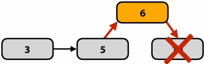
Solution 1: protect the list with a single lock
1 | struct Node { |
Single global lock per data structure
Good:
It is relatively simple to implement correct mutual exclusion for data structure operations (we just did it!)
Bad:
Operations on the data structure are serialized
May limit parallel application performance
Solution 2: “hand-over-hand” locking fine-grained locking
1 | struct Node { |
Challenge to students: there is way to further improve the implementation of insert(). What is it?
由于持有 prev 的锁足以阻止任何可能导致 cur 节点失效的操作(如删除),因此 insert() 在遍历和执行插入时,只需要持有 prev 的锁,无需锁定 cur
Fine-grained locking
Goal: enable parallelism in data structure operations
Reduces contention for global data structure lock
In the linked-list example: a single monolithic(整体式) lock is overly conservative (operations on different parts of the linked list can proceed in parallel)
Challenge: tricky to ensure correctness
Determining when mutual exclusion is required
Deadlock?
Livelock?
Costs?
Overhead of taking a lock each traversal step (extra instructions + traversal now involves memory writes)
Extra storage cost (a lock per node)
What is a middle-ground solution that trades off some parallelism for reduced overhead? (hint: similar issue to selection of task granularity)
多个节点一个锁
Practice exercise (on your own time)
Implement a fine-grained locking implementation of a binary search tree supporting insert and delete
1 | struct Tree { |
Using locks: Lock-free data structure designs
Blocking algorithms/data structures
A blocking algorithm allows one thread to prevent other threads from completing operations on a shared data structure indefinitely
Example:
Thread 0 takes a lock on a node in our linked list
Thread 0 is swapped out by the OS, or crashes, or is just really slow (takes a page fault), etc
Now, no other threads can complete operations on the data structure (although thread 0 is not actively making progress modifying it)
An algorithm that uses locks is blocking regardless of whether the lock implementation uses spinning or pre-emption(抢占)
Lock-free algorithms
Non-blocking algorithms are lock-free if some thread is guaranteed to make progress (“systemwide progress”)
In lock-free case, it is not possible to preempt(抢占) one of the threads at an inopportune(不合时宜) time and prevent progress by rest of system
Note: this definition does not prevent starvation of any one thread
Single reader, single writer bounded queue
Assume a sequentially consistent memory system for now (or the presence of appropriate memory fences, or C++ 11 atomic<>)
Only two threads (one producer, one consumer) accessing queue at the same time
Threads never synchronize or wait on each other
When queue is empty (pop fails), when it is full (push fails)
1 | struct Queue { |
Single reader, single writer unbounded queue
Assume a sequentially consistent memory system for now (or the presence of appropriate memory fences, or C++ 11 atomic<>)
Tail points to last element added (if non-empty)
Head points to element BEFORE head of queue
Node allocation and deletion performed by the same thread (producer thread)
1 | struct Node { |
Lock-free stack (first try)
Assume a sequentially consistent memory system for now (or the presence of appropriate memory fences, or C++ 11 atomic<>)
Main idea: as long as no other thread has modified the stack, a thread’s modification can proceed
Note difference from fine-grained locking: In fine-grained locking, the implementation locked a part of a data structure. Here, threads do not hold lock on data structure at all
1 | struct Node { |
The ABA problem
Careful: A, B, C, and D are addresses of nodes, not the value stored by the nodes!
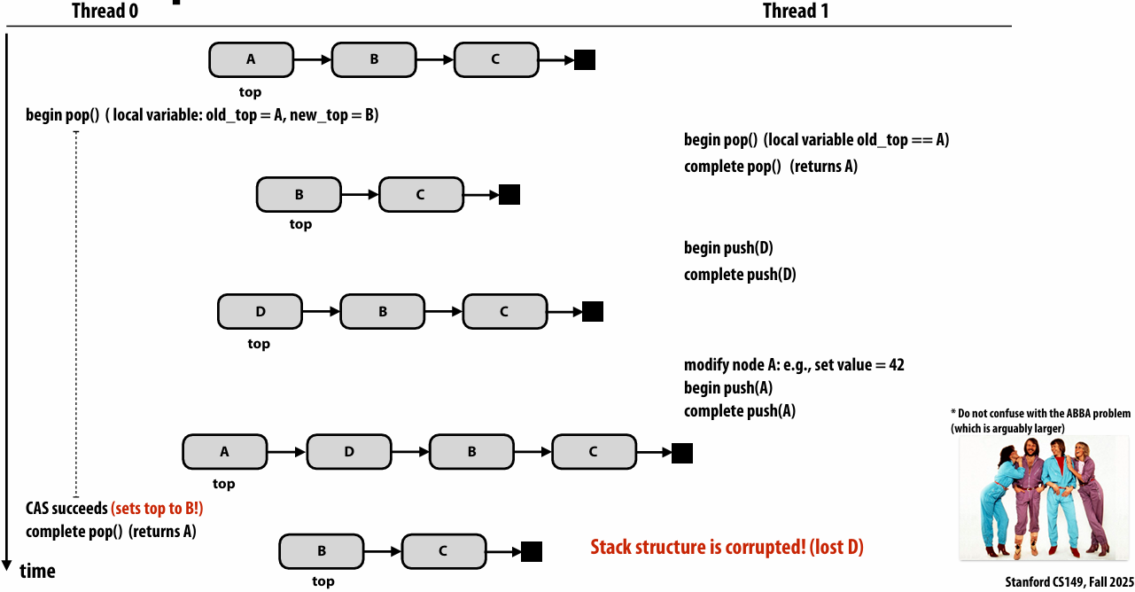
ABBA 问题 (死锁): ABBA 形象地描述了两个线程尝试以相反的顺序获取两把锁的情况
Lock-free stack using counter for ABA soln
Maintain counter of pop operations
Requires machine to support “double compare and swap” (DCAS) or doubleword CAS
Could also solve ABA problem with careful node allocation and/or element reuse policies
1 | struct Node { |
Compare and swap on x86
x86 supports a “double-wide” compare-and-swap instruction
Not quite the “double compare-and-swap” used on the previous
But could simply ensure the stack’s count and top fields are contiguous in memory to use the 64-bit wide single compare-and-swap instruction below
cmpxchg8b
“compare and exchange eight bytes”
Can be used for compare-and-swap of two 32-bit values
cmpxchg16b
“compare and exchange 16 bytes”
Can be used for compare-and-swap of two 64-bit values
Another problem: referencing freed memory
1 | struct Node { |
[Advanced topic] Hazard pointer: avoid freeing a node until it’s known that all other threads do not hold reference to it
1 | struct Node { |
Lock-free linked list insertion
For simplicity, this slide assumes the only operation on the list is insert. Delete is more complex
Compared to fine-grained locking implementation:
No overhead of taking locks
No per-node storage overhead
1 | struct Node { |
Lock-free linked list deletion
Supporting lock-free deletion significantly complicates data-structure
Consider case where B is deleted simultaneously with insertion of E after B
B now points to E, but B is not in the list!
For the curious:
Harris 2001. “A Pragmatic Implementation of Non-blocking Linked-Lists”
Fomitchev 2004. “Lock-free linked lists and skip lists”
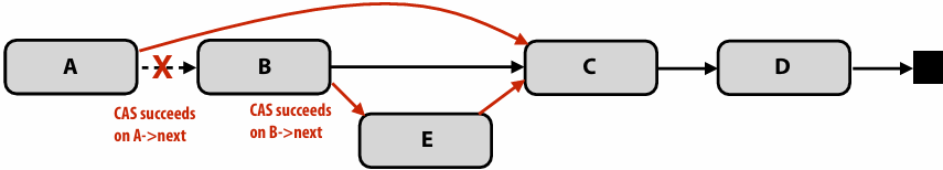
Lock-free vs. locks performance comparison
Lock-free algorithm run time normalized to run time of using pthread mutex locks
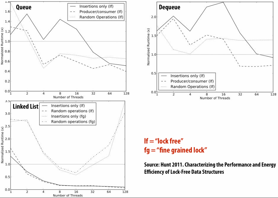
In practice: why lock free data structures?
When optimizing parallel programs in this class you often assume that only your program is using the machine
Because you care about performance
Typical assumption in scientific computing, graphics, machine learning, data analytics, etc.
In these cases, well-written code with locks can be as fast (or faster) than lock-free code
And is often much simpler to implement
But there are situations where code with locks can suffer from tricky performance problems
Situations where a program features many threads (e.g., database, webserver) and page faults, pre-emption, etc. can occur while a thread is in a critical section
Locks create problems like priority inversion(反转), convoying, crashing in critical section, etc. that are often discussed in OS classes
Summary
Use fine-grained locking to reduce contention (maximize parallelism) in operations on shared data structures
But fine-granularity can increase code complexity (errors) and increase execution overhead
Lock-free data structures: non-blocking solution to avoid some overheads/pitfalls(陷阱) of locks
But can be tricky to implement (and ensuring correctness in a lock-free setting has its own overheads)
Still requires appropriate memory fences on modern relaxed consistency hardware
Note: a lock-free design does not eliminate contention
Compare-and-swap can fail under heavy contention, requiring spins
Preview: transactional memory
Q. What was the role of the compare and swap in our lock-free implementations?
A. Determining if another thread had modified the data structure while the calling thread was in the middle of an operation
Next time… transactional memory
A more general mechanism to allow a system to speculate that an operation will be successfully completed before another thread attempts to modify the structure
With mechanisms to “abort” an operation in the event another thread does
More reading on lock-free structures
Michael and Scott 1996. Simple, Fast and Practical Non-Blocking and Blocking Concurrent Queue Algorithms
Multiple reader/writer lock-free queue
Harris 2001. A Pragmatic(实用) Implementation of Non-Blocking Linked-Lists
Michael Sullivan’s Relaxed Memory Calculus (RMC) compiler
msullivan/rmc-compiler: Implementation of RMC atomics for C/C++
Many good blog posts and articles on the web:
http://www.drdobbs.com/cpp/lock-free-code-a-false-sense-of-security/210600279
developers.memsql.com
Lecture 17: Transactional Memory
Transactional Memory (TM) Semantics
Raising level of abstraction for synchronization
Previous topic: machine-level atomic operations
Test-and-set, fetch-and-op, compare-and-swap, load linked-store conditional
Then we used these atomic operations to construct higher level synchronization primitives in software:
Locks, barrier
Lock-free data structures
We’ve seen how it can be challenging to produce correct programs using these primitives (easy to create bugs that violate atomicity, create deadlock, etc.)
Today: raising level of abstraction for synchronization even further
Idea: transactional memory
What you should know
What a transaction is
The difference (in semantics) between an atomiccode block and lock/unlock primitives
The basic design space of transactional memory implementations
Data versioning policy
Conflict detection policy
Granularity of detection
The basics of a software implementation of transactional memory
The basics of a hardware implementation of transactional memory (consider how it relates to the cache coherence protocol implementations we’ve discussed previously in the course)
Between a Lock and a Hard Place
Locks force trade-off between
Degree of concurrency ⇒ performance
Chance of races, deadlock ⇒ correctness
Coarse grain locking
low concurrency, higher chance of correctness
E.g. single lock for the whole data structure or all shared memory
Fine grain locking
high concurrency, lower chance of correctness
E.g. hand-over-hand locking
Is there a better synchronization abstraction?
Review: ensuring atomicity via locks
1 | void deposit(Acct account, int amount) |
Deposit is a read-modify-write operation: want “deposit” to be atomic with respect to other bank operations on this account
Locks are one mechanism to synchronize threads to ensure atomicity of update (via ensuring mutual exclusion on the account)
Programming with transactions
1 | void deposit(Acct account, int amount) |
Atomic construct is declarative
Programmer states what to do (maintain atomicity of this code), not how to do it
No explicit use or management of locks
System implements synchronization as necessary to ensure atomicity
System could implement atomic { } using locks
Implementation discussed today uses optimistic concurrency: maintain serialization only in situations of true contention (R-W or W-W conflicts)
Declarative vs. Imperative(命令式) Abstractions
Declarative: programmer defines what should be done
Execute all these independent 1000 tasks
Perform this set of operations atomically
Imperative: programmer states how it should be done
Spawn N worker threads. Assign work to threads by removing work from a shared task queue
Acquire a lock, perform operations, release the lock
Transactional Memory (TM) Semantics
Memory transaction
An atomic and isolated sequence of memory accesses
Inspired by database transactions
Atomicity (all or nothing)
Upon transaction commit, all memory writes in transaction take effect at once
On transaction abort, none of the writes appear to take effect (as if transaction never happened)
Isolation
No other processor can observe writes before transaction commits
Serializability
Transactions appear to commit in a single serial order
But the exact order of commits is not guaranteed by semantics of transaction
Transactional Memory (TM)
In other words… many of the properties we maintained for a single address in a coherent memory system, we’d like to maintain for sets of reads and writes in a transaction
Transaction:
Reads: X, Y, Z
Writes: A, X
These memory transactions will either all be observed by other processors, or none of them will. (the effectively all happen at the same time)
What is the consistency model for TM?
It gives you basically sequential consistency, some people have called this transactional consistency
Motivating transactional memory
Java HashMap
Map: Key → Value
Implemented as a hash table with linked list per bucket
1 | public Object get(Object key) { |
Bad: not thread safe (when synchronization needed)
Good: no lock overhead when synchronization not needed
Synchronized HashMap
Java 1.4 solution: synchronized layer
Convert any map to thread-safe variant
Uses explicit, coarse-grained mutual locking specified by programmer
1 | public Object get(Object key) { |
Coarse-grain synchronized HashMap
Good: thread-safe, easy to program
Bad: limits concurrency, poor scalability
One solution: use finer-grained synchronization (e.g., lock per bucket)
Now thread safe: but incurs lock overhead even if synchronization not needed
performance of fine-grained locking
Reducing contention via fine-grained locking leads to better performance
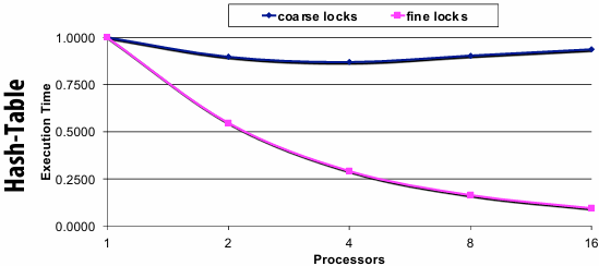
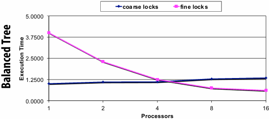
Transactional HashMap
Simply enclose all operation in atomic block
Semantics of atomic block: system ensures atomicity of logic within block
1 | public Object get(Object key) { |
Good: thread-safe, easy to program
What about performance and scalability?
Depends on the workload and implementation of atomic (to be discussed)
Another example: tree update by two threads
Goal: modify nodes 3 and 4 in a thread-safe way
Fine-grained locking example
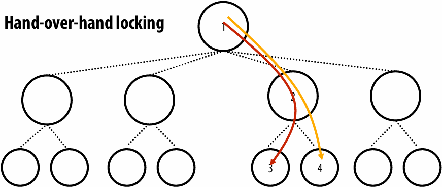
Locking can prevent concurrency (here: locks on node 1 and 2 during update to node 3 could delay update to 4)
Transactions example
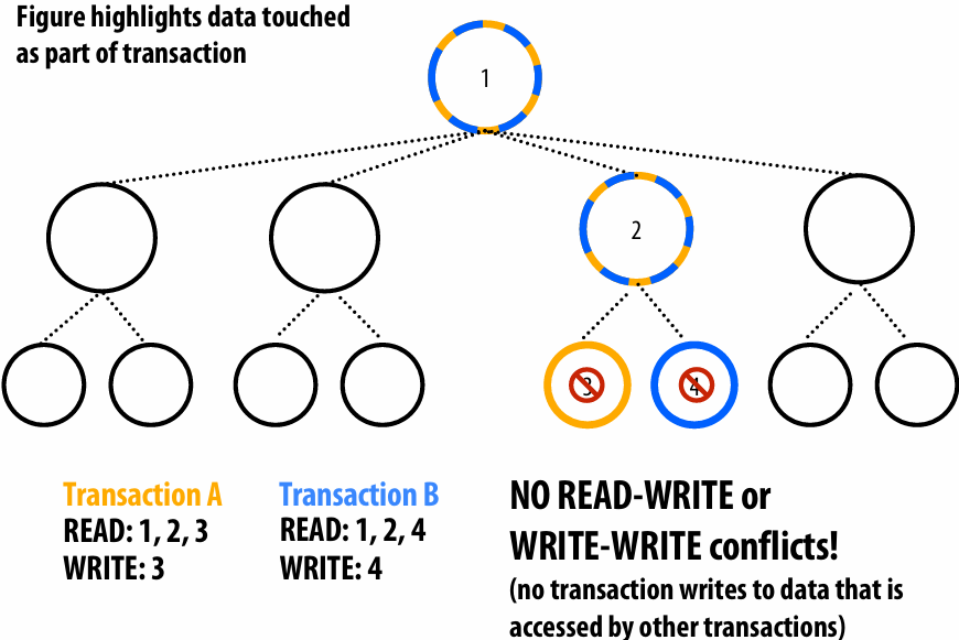
Transactions example #2
(Both transactions modify node 3)
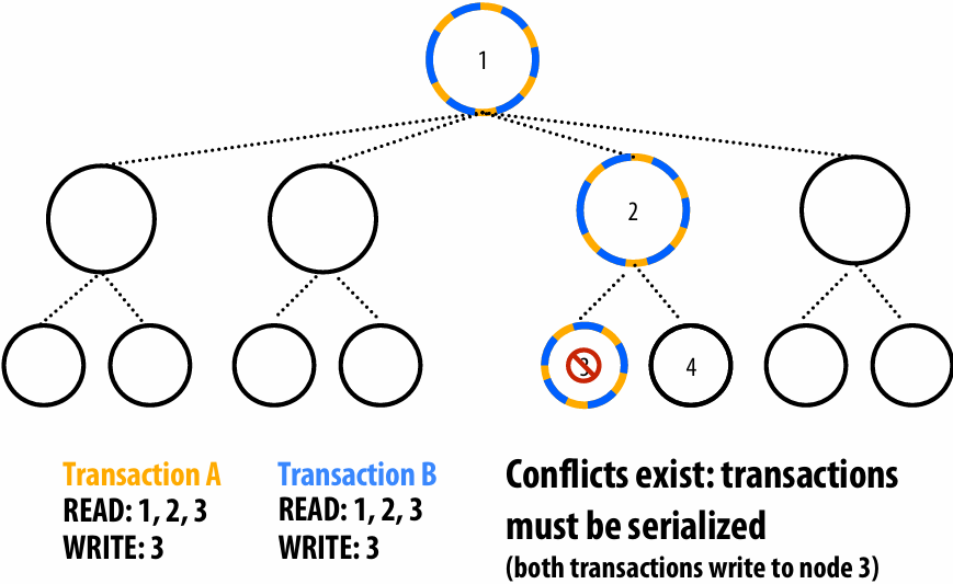
Performance: locks vs. transactions
HashMap Balanced Tree
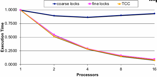
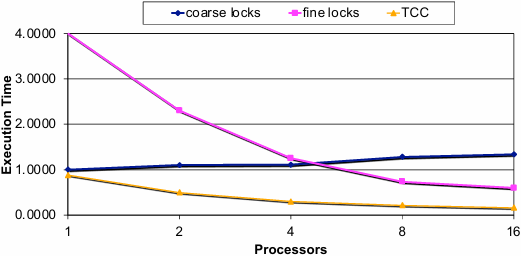
“TCC” is a TM system implemented in hardware
Atomic and Doubly-Linked List
Make PushLeft method on a doubly-linked list thread safe using atomic()
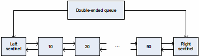
1 | void PushLeft(DQueue *q, int val) { |
Another motivation: failure atomicity
Failure atomicity: locks
1 | void transfer(A, B, amount) { |
Complexity of manually catching exceptions
Programmer provides “undo” code on a case-by-case(具体情况) basis
Complexity: must track what to undo and how…
Some side-effects may become visible to other threads
E.g., an uncaught case can deadlock the system…
Failure atomicity: transactions
1 | void transfer(A, B, amount) |
System now responsible for processing exceptions
All exceptions (except those explicitly managed by the programmer)
Transaction is aborted and memory updates are undone
Recall: a transaction either commits or it doesn’t: no partial updates are visible to other threads
E.g., no locks held by a failing threads…
Another motivation: composability
Composability: locks
1 | void transfer(A, B, amount) |
DEADLOCK!
Thread 0: transfer(A, B, 100)
Thread 1: transfer(B, A, 200)
Composing lock-based code can be tricky
Requires system-wide policies to get correct
System-wide policies can break software modularity
Programmer caught between a lock and a hard place !
Coarse-grain locks: low performance
Fine-grain locking: good for performance, but mistakes can lead to deadlock
Composability: transactions
1 | void transfer(A, B, amount) { |
Transactions compose gracefully (in theory)
Programmer declares global intent(意图) (atomic execution of transfer)
No need to know about global implementation strategy
Transaction in transfer subsumes(包含) any defined in withdraw and deposit
Outermost transaction defines atomicity boundary
System manages concurrency as well as possible
Serialization for transfer(A, B, 100) and transfer(B, A, 200)
Concurrency for transfer(A, B, 100) and transfer(C, D, 200)
Advantages (promise) of transactional memory
Easy to use synchronization construct
It is difficult for programmers to get synchronization right
Programmer declares need for atomicity, system implements it well
Claim: transactions are as easy to use as coarse-grain locks
Often performs as well as fine-grained locks
Provides automatic read-read concurrency and fine-grained concurrency
Performance portability: locking scheme for four CPUs may not be the best scheme for 64 CPUs
Productivity argument for transactional memory: system support for transactions can achieve 90% of the benefit of expert programming with fined-grained locks, with 10% of the development time
Failure atomicity and recovery
No lost locks when a thread fails
Failure recovery = transaction abort + restart
Composability
Safe and scalable composition of software modules
Self-check: atomic { } ≠ lock() + unlock()
The difference (Make sure you understand this difference in semantics!)
Atomic: high-level declaration of atomicity
Does not specify implementation of atomicity
Lock: low-level blocking primitive
Does not provide atomicity or isolation on its own
Keep in mind
Locks can be used to implement an atomicblock but…
Locks can be used for purposes beyond atomicity
Cannot replace all uses of locks with atomic regions
Atomic eliminates many data races, but programming with atomic blocks can still suffer from atomicity violations: e.g., programmer erroneous splits sequence that should be atomic into two atomic blocks
What about replacing synchronized with atomic in this example?
1 | // Thread 1 |
Thread 1 和 Thread 2 读区域和写区域相互冲突,导致序列化执行,又因为无法满足 while 循环条件,导致先执行的线程死循环
Atomicity violation due to programmer error
1 | // Thread 1 |
Programmer mistake: logically atomic code sequence (in thread 1) is erroneously separated into two atomic blocks (allowing another thread to set pointer to NULL in between)
Implementing transactional memory
Recall transactional semantics
Atomicity (all or nothing)
At commit, all memory writes take effect at once
In event of abort, none of the writes appear to take effect
Isolation
No other code can observe writes before commit
Serializability
Transactions seem to commit in a single serial order
The exact order is not guaranteed though
TM implementation basics
TM systems must provide atomicity and isolation
While maintaining as much concurrency as possible
Two key implementation questions
Data versioning policy: How does the system manage uncommitted (new) and previously committed (old) versions of data for concurrent transactions?
Conflict detection policy: how/when does the system determine that two concurrent transactions conflict?
Data versioning policy
Manage uncommitted (new) and previously committed (old) versions of data for concurrent transactions
1.Eager versioning (undo-log based)
2.Lazy versioning (write-buffer based)
Eager versioning
Update memory immediately, maintain “undo log” in case of(以防) abort
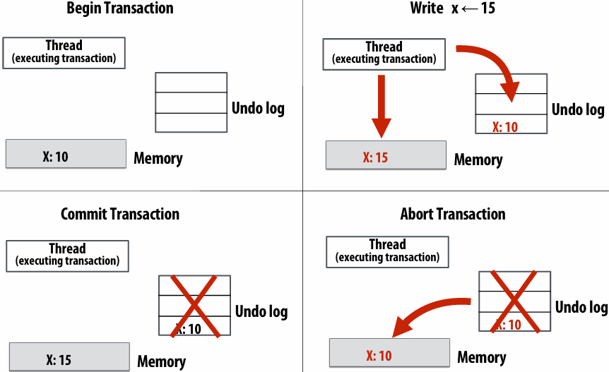
Lazy versioning
Log memory updates in transaction write buffer, flush buffer on commit
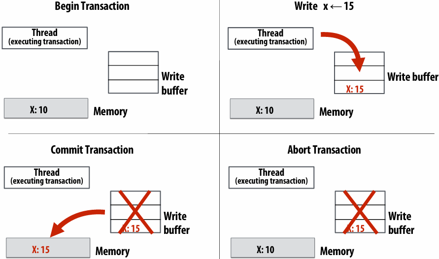
Data versioning
Goal: manage uncommitted (new) and committed (old) versions of data for concurrent transactions
Eager versioning (undo-log based)
Update memory location directly on write
Maintain undo information in a log (incurs per-store overhead)
Good: faster commit (data is already in memory)
Bad: slower aborts, fault tolerance issues (consider crash in middle of transaction)
Eager versioning philosophy: write to memory immediately, hoping transaction won’t abort (but deal with aborts when you have to)
Lazy versioning (write-buffer based)
Buffer data in a write buffer until commit
Update actual memory location on commit
Good: faster abort (just clear log), no fault tolerance issues
Bad: slower commits
Lazy versioning philosophy: only write to memory when you have to
Conflict detection
Must detect and handle conflicts between transactions
Read-write conflict: transaction A reads address X, which was written to by pending(待办的) (but not yet committed) transaction B
Write-write conflict: transactions A and B are both pending, and both write to address X
System must track a transaction’s read set and write set
Read-set: addresses read during the transaction
Write-set: addresses written during the transaction
Pessimistic detection
Check for conflicts (immediately) during loads or stores
Philosophy: “I suspect conflicts might happen, so let’s always check to see if one has occurred after each memory operation… if I’m going to have to roll back, might as well do it now to avoid wasted work.”
“Contention manager” decides to stall or abort transaction when a conflict is detected
Various policies to handle common case fast
Pessimistic detection examples
Note: diagrams assume “aggressive” contention manager on writes: writer wins, so other transactions abort)
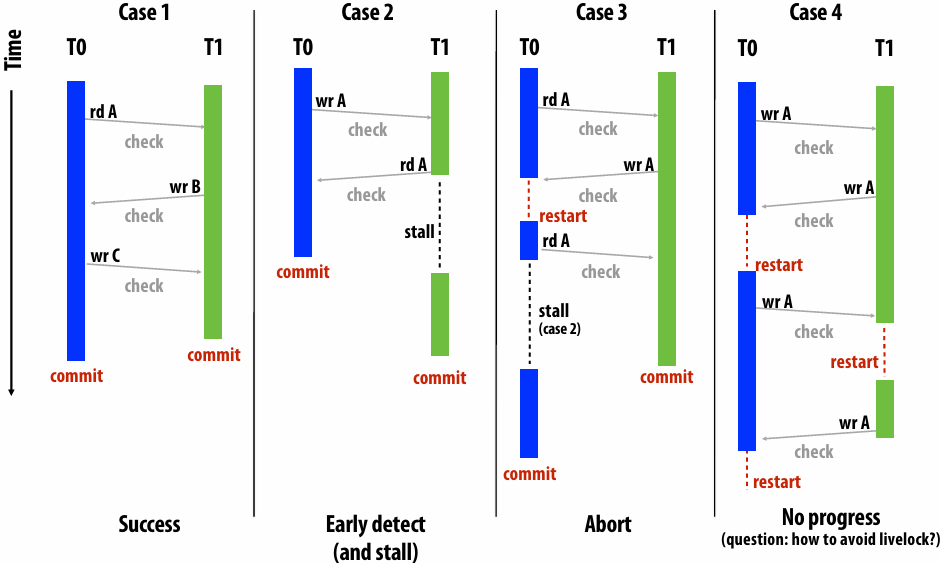
Optimistic detection
Detect conflicts when a transaction attempts to commit
Intuition: “Let’s hope for the best and sort out(解决) all the conflicts only when the transaction tries to commit”
On a conflict, give priority to committing transaction
Other transactions may abort later on
Optimistic detection examples
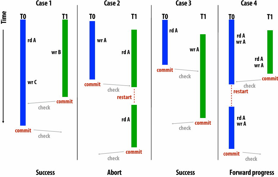
Conflict detection trade-offs
Pessimistic conflict detection (a.k.a. “eager”)
Good: detect conflicts early (undo less work, turn some aborts to stalls)
Bad: no forward progress guarantees, more aborts in some cases
Bad: fine-grained communication (check on each load/store)
Bad: detection on critical path
Optimistic conflict detection (a.k.a.“lazy” or “commit”)
Good: forward progress guarantees
Good: bulk communication and conflict detection
Bad: detects conflicts late, can still have fairness problems
Lecture 18: Transactional Memory Part II + Course Wrap Up
TM implementation space (examples)
Software TM systems
Lazy + optimistic (rd/wr): Sun TL2
Lazy + optimistic (rd)/pessimistic (wr): MS OSTM
Eager + optimistic (rd)/pessimistic (wr): Intel STM
Eager + pessimistic (rd/wr): Intel STM
Hardware TM systems
Lazy + optimistic: Stanford TCC
Lazy + pessimistic: MIT LTM, Intel VTM
Eager + pessimistic: Wisconsin LogTM (easiest with conventional cache coherence)
Optimal design remains an open question
May be different for HW, SW, and hybrid
Software TM systems
Software Transactional Memory
1 | atomic { |
Software barriers (STM function call) for TM bookkeeping
Versioning, read/write-set tracking, commit, …
Using locks, timestamps, data copying, …
Requires function cloning or dynamic translation
Function used inside and outside of transaction
STM Runtime Data Structures
Transaction descriptor (per-thread)
Used for conflict detection, commit, abort, …
Includes the read set, write set, undo log or write buffer
Transaction record (per data)
Pointer-sized record guarding shared data
Tracks transactional state of data
Shared: accessed by multiple readers
Using version number or shared reader lock
Exclusive: access by one writer
Using writer lock that points to owner
BTW(顺便提一句): same way that HW cache coherence works
Mapping Data to Transaction Records
Every data item has an associated transaction record
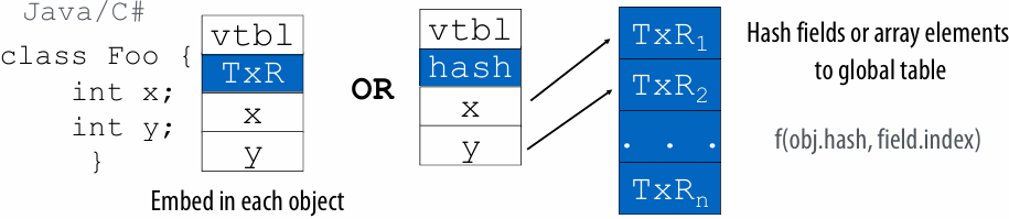
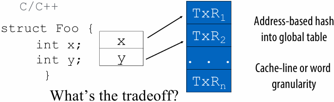
Conflict Detection Granularity
Object granularity
Low overhead mapping operation
Exposes optimization opportunities
False conflicts (e.g. Txn 1 and Txn 2)
Element/field granularity (word)
Reduces false conflicts
Improves concurrency (e.g. Txn 1 and Txn 2)
Increased overhead (time/space)
Cache line granularity (multiple words)
Matches hardware TM
Reduces storage overhead of transactional records
Hard for programmer & compiler to analyze
Mix & match per type basis
E.g., element-level for arrays, object-level for non-arrays
1 | // Txn 1 |
An Example STM Algorithm
Based on Intel’s McRT STM [PPoPP’06, PLDI’06, CGO’07]
Eager versioning, optimistic reads, pessimistic writes
Based on timestamp for version tracking
Global timestamp
Incremented when a writing xaction commits
Local timestamp per xaction
Global timestamp value when xaction last validated
Transaction record (32-bit)
LS bit: 0 if writer-locked, 1 if not locked
MS bits
Timestamp (version number) of last commit if not locked
Pointer to owner xaction if locked
STM Operations
STM read (optimistic)
Direct read of memory location (eager)
Validate read data
Check if unlocked and data version ≤ local timestamp
If not, validate all data in read set for consistency
Insert in read set
Return value
STM write (pessimistic)
Validate data
Check if unlocked and data version ≤ local timestamp
Acquire lock
Insert in write set
Create undo log entry
Write data in place (eager)
STM Operations (cont)
Read-set validation
Get global timestamp
For each item in the read set
If locked by other or data version > local timestamp, abort
Set local timestamp to global timestamp from initial step
STM commit
Atomically increment global timestamp by 2 (LSb used for write-lock)
If preincremented (old) global timestamp > local timestamp, validate read-set
Check for recently committed transactions
For each item in the write set
Release the lock and set version number to global timestamp
STM Example
1 | // X1 |
X1 copies object foo into object bar
X2 should read bar as [0,0] or [9,7]
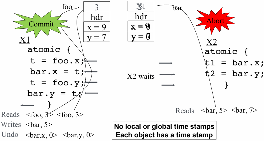
TM Implementation Summary 1
TM implementation
Data versioning: eager or lazy
Conflict detection: optimistic or pessimistic
Granularity: object, word, cache-line, …
Software TM systems
Compiler adds code for versioning & conflict detection
Note: STM barrier = instrumentation code
Basic data-structures
Transactional descriptor per thread (status, rd/wr set, …)
Transactional record per data (locked/version)
Challenges for STM Systems
Overhead of software barriers
Function cloning
Robust(稳健的) contention management
Memory model (strong Vs. weak atomicity)
Optimizing Software Transactions
Monolithic(整体式) barriers hide redundant logging & locking from the compiler
1 | atomic { |
Decomposed barriers expose redundancies
1 | atomic { |
Allows compiler to optimize STM code
Produces fewer & cheaper STM operations
1 | atomic { |
Effect of Compiler Optimizations
1 thread overheads over(相对于) thread-unsafe baseline
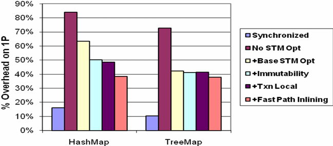
With compiler optimizations
<40% over no concurrency control
<30% over lock-based synchronization
STM Question
Given an optimistic read, pessimistic write, eager versioning STM
What steps are required to implement the atomic region
1 | atomic{ |
1 | tx = GetTxDescriptor(); // Assume a way of to get transaction descriptor |
Hardware TM systems
Motivation for Hardware Support
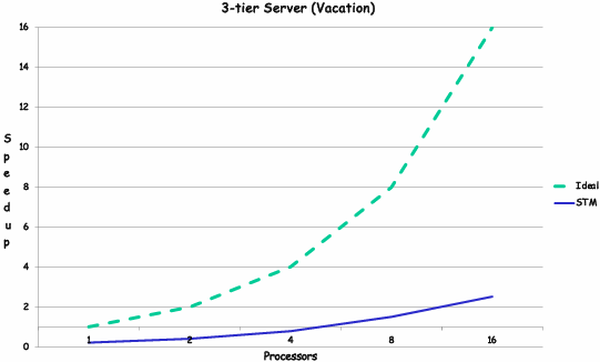
STM slowdown: 2-8x per thread overhead due to barriers
Short term issue: demotivates parallel programming
Long term issue: energy wasteful
Lack of strong atomicity
Costly to provide purely in software
Why is STM Slow?
Measured single-thread STM performance
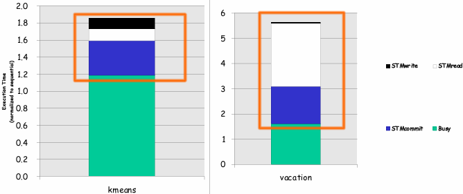
1.8x – 5.6x slowdown over sequential
Most time goes in read barriers & commit
Most apps read more data than they write
Types of Hardware Support
Hardware-accelerated STM systems (HASTM, SigTM, USTM, …)
Start with an STM system & identify key bottlenecks
Provide (simple) HW primitives for acceleration, but keep SW barriers
Hardware-based TM systems (TCC, LTM, VTM, LogTM, …)
Versioning & conflict detection directly in HW
No SW barriers
Hybrid TM systems (Sun Rock, …)
Combine an HTM with an STM by switching modes when needed
Based on xaction characteristics available resources, …
| HTM | STM | HW-STM | |
|---|---|---|---|
| Write versioning | HW | SW | SW |
| Conflict detection | HW | SW | HW |
Hardware transactional memory (HTM)
Data versioning is implemented in caches
Cache the write buffer or the undo log
Add new cache line metadata to track transaction read set and write set
Conflict detection through cache coherence protocol
Coherence lookups detect conflicts between transactions
Works with snooping and directory coherence
Note:
Register checkpoint must also be taken at transaction begin (to restore execution context state on abort)
HTM design
Cache lines annotated(带注释的) to track read set and write set
R bit: indicates data read by transaction (set on loads)
W bit: indicates data written by transaction (set on stores)
R/W bits can be at word or cache-line granularity
R/W bits gang-cleared(集体清除) on transaction commit or abort
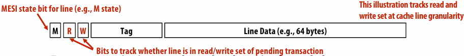
For eager versioning, need a 2nd cache write for undo log
Coherence requests check R/W bits to detect conflicts
Observing shared request to W-word is a read-write conflict
Observing exclusive (intent to write) request to R-word is a write-read conflict
Observing exclusive (intent to write) request to W-word is a write-write conflict
Example HTM implementation: lazy-optimistic
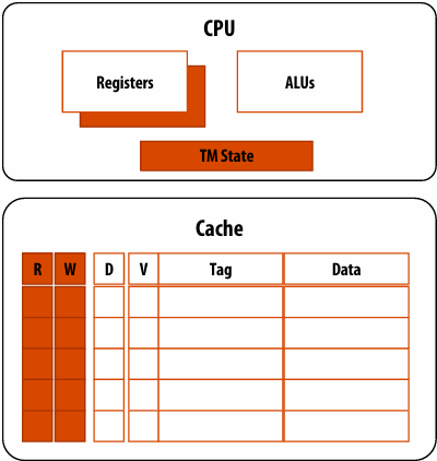
CPU changes
Ability to checkpoint register state (available in many CPUs)
TM state registers (status, pointers to abort handlers, …)
Cache changes
R bit indicates membership to read set
W bit indicates membership to write set
HTM transaction execution
1 | Xbegin |
Transaction begin Xbegin
Initialize CPU and cache state
Take register checkpoint
Load operation Load A Load B
Serve cache miss if needed
Mark data as part of read set
Store operation Store C ⇐ 5
Service cache miss if needed
Mark data as part of write set (note: this is not a load into exclusive state. Why?)
That each of these transactions is isolated from each other
Fast two-phase commit
Validate: request RdX access to write set lines (if needed)
Commit: gang-reset R and W bits, turns write set data to valid (dirty) data
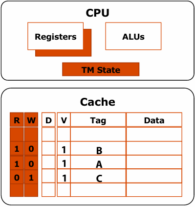
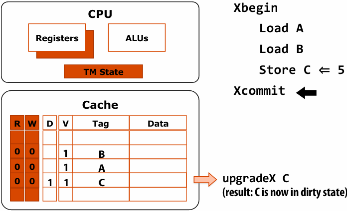
HTM transaction execution: detect/abort
Assume remote processor commits transaction with writes to A and D
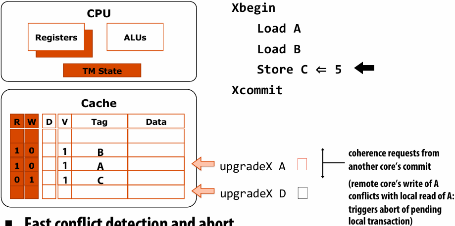
Fast conflict detection and abort
Check: lookup exclusive requests in the read set and write set
Abort: invalidate write set, gang-reset R and W bits, restore to register checkpoint
HTM Performance Example
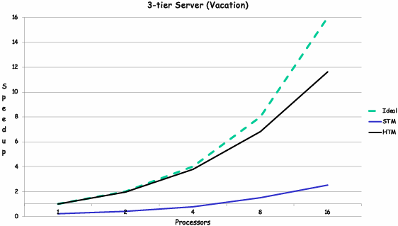
2x to 7x over STM performance
Within 10% of sequential for one thread
Scales efficiently with number of processors
HTM Example: Transactional Coherence and Consistency
Use TM as the coherence mechanism -> all transactions all the time
Successful transaction commits update memory and all caches in the system
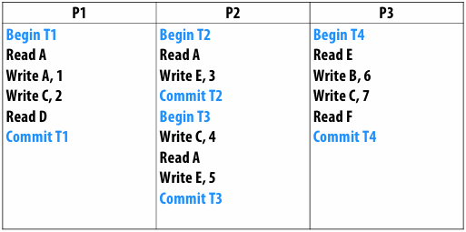
Assumptions
Lazy and optimistic
One “commit” per execution step across all processors
When one transaction causes another transaction to abort and re-execute, assume that the transaction “commit” of one transaction can overlap with the “begin” of the re-executing transaction
Minimize the number of execution steps
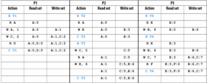
Hardware transactional memory support in Intel Haswell architecture
New instructions for “restricted transactional memory” (RTM)
xbegin: takes pointer to “fallback(倒退) address” in case of abort
e.g., fallback to code-path with a spin-lock
xend
xabort
Implementation: tracks read and write set in L1 cache
Processor makes sure all memory operations commit atomically
But processor may automatically abort transaction for many reasons (e.g., eviction(驱逐) of line in read or write set will cause a transaction abort)
Implementation does not guarantee progress (see fallback address)
Intel optimization guide (ch 12) gives guidelines for increasing probability(可能性) that transactions will not abort
Summary: transactional memory
Atomic construct: declaration that atomic behavior must be preserved by the system
Motivating idea: increase simplicity of synchronization without (significantly) sacrificing(牺牲) performance
Transactional memory implementation
Many variants have been proposed: SW, HW, SW+HW
Implementations differ in:
Data versioning policy (eager vs. lazy)
Conflict detection policy (pessimistic vs. optimistic)
Detection granularity (object, word, cache line)
Software TM systems (STM)
Compiler adds code for versioning & conflict detection
Note: STM barrier = instrumentation code (e.g. StmRead, StmWrite)
Basic data-structures
Transactional descriptor per thread (status, rd/wr set, …)
Transactional record per data (locked/version)
Hardware Transactional Memory (HTM)
Versioned data is kept in caches
Conflict detection mechanisms augment(增强) coherence protocol
Course Wrap Up
For the foreseeable future, the primary way to obtain higher performance computing hardware is through a combination of increased parallelism and hardware specialization
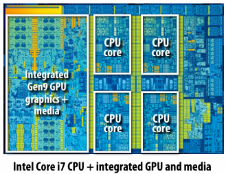
Modern software is surprisingly inefficient compared to the peak capability of modern machines
A lot of performance is currently left on the table (increasingly so as machines get more complex, and parallel processing capability grows)
Extracting this performance stands to provide a notable impact on many compute-intensive fields (or, more importantly enable new applications of computing!)
Given current software programming systems and tools, understanding principles of how a parallel machine works is important to achieving high performance
A major challenge going forward is making it simpler for programmers to extract performance on these complex machines
This is very important given how exciting (and efficiency-critical) the next generation of computing applications are likely to be

Key issues we have addressed in this course
Identifying parallelism
(or conversely, identifying dependencies)
Efficiently scheduling work
1.Achieving good workload balance
2.Overcoming communication constraints:
Bandwidth limits, dealing with latency, synchronization
Exploiting data/computation locality = efficiently managing state!
3.Scheduling under heterogeneity (using the right processor for the job)
We discussed these issues at many scales and in many contexts
Heterogeneous mobile SoC
Single chip, multi-core CPU
Multi-core GPU
CPU+GPU connected via bus
Clusters of machines
AI accelerator hardware
Large scale, multi-node supercomputers
How throughput-oriented hardware works
Multiple cores, hardware-threads, SIMD
Specialized AI accelerators
Specialization to key domains
Abstractions that help structure code to be efficient
Data parallel thinking
Functional parallelism
Transactions
Tasks
SPMD
Other relevant classes
CS 217: Hardware Accelerators for Machine Learning (Winter, Kunle’s course)
Focuses on design of specialized hardware architectures for ML (understanding the workload and building efficient hardware for that workload)
CS 348K: Visual Computing Systems (Spring, Kayvon)
Design of high-performance hardware/software systems for processing images and video (ray tracing, video analysis, smartphone camera processing, NeRF/AI-based graphics, fast data labeling, etc)
CS/EE 282: Computer Systems Architecture
- Titre: 【Class】Stanford CS149 Parallel Computing
- Auteur: tiny_star
- Créé à : 2025-12-25 01:04:13
- Mis à jour à : 2026-03-02 23:12:46
- Lien: https://tiny-star3.github.io/2025/12/25/Cpp/[Class]Stanford CS149 Parallel Computing/
- Licence: Cette œuvre est sous licence CC BY-NC-SA 4.0.